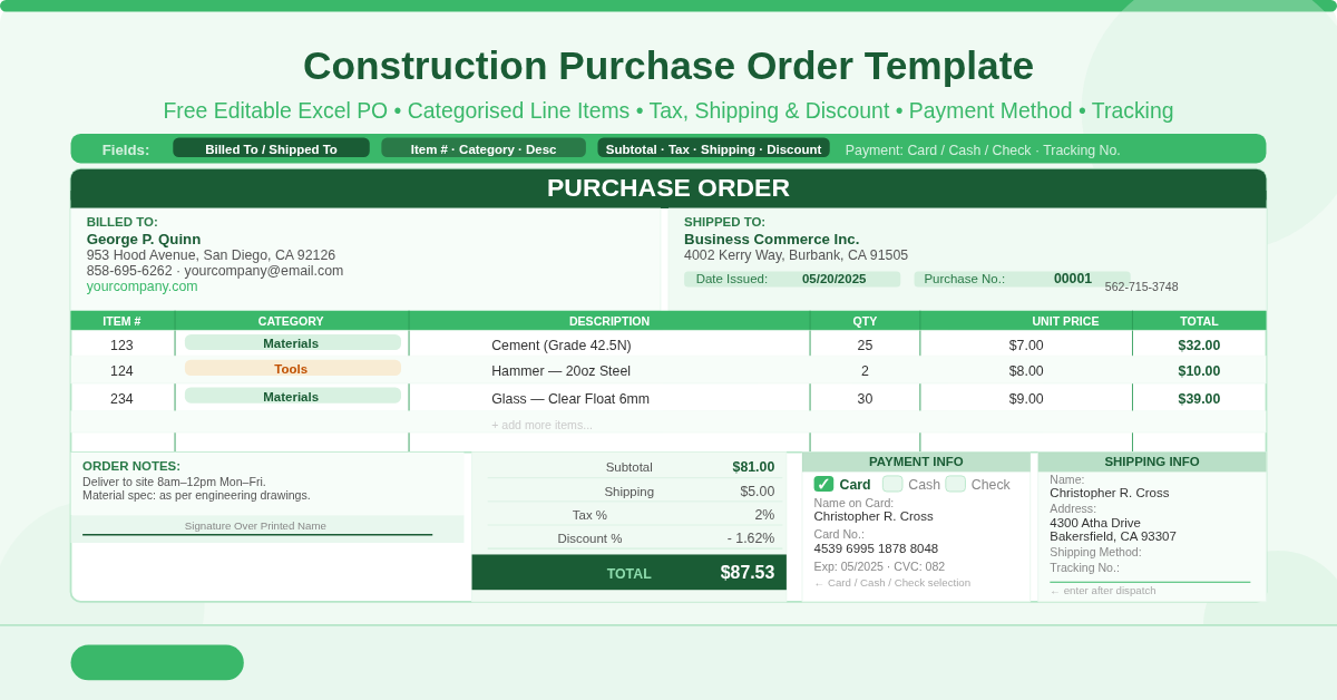
Construction Purchase Order
A free editable Excel construction purchase order template with categorised line items, tax, shipping, discount, payment method selection, and shipping tracking — print-ready for any job.
A free editable Excel construction purchase order template with categorised line items, tax, shipping, discount, payment method selection, and shipping tracking — print-ready for any job.
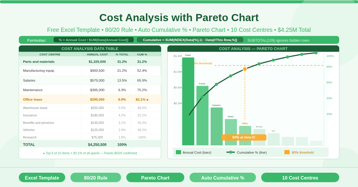
A free Excel Pareto chart cost analysis template that ranks cost centres by spend, calculates cumulative percentages automatically, and reveals the 20% driving 80% of your costs.
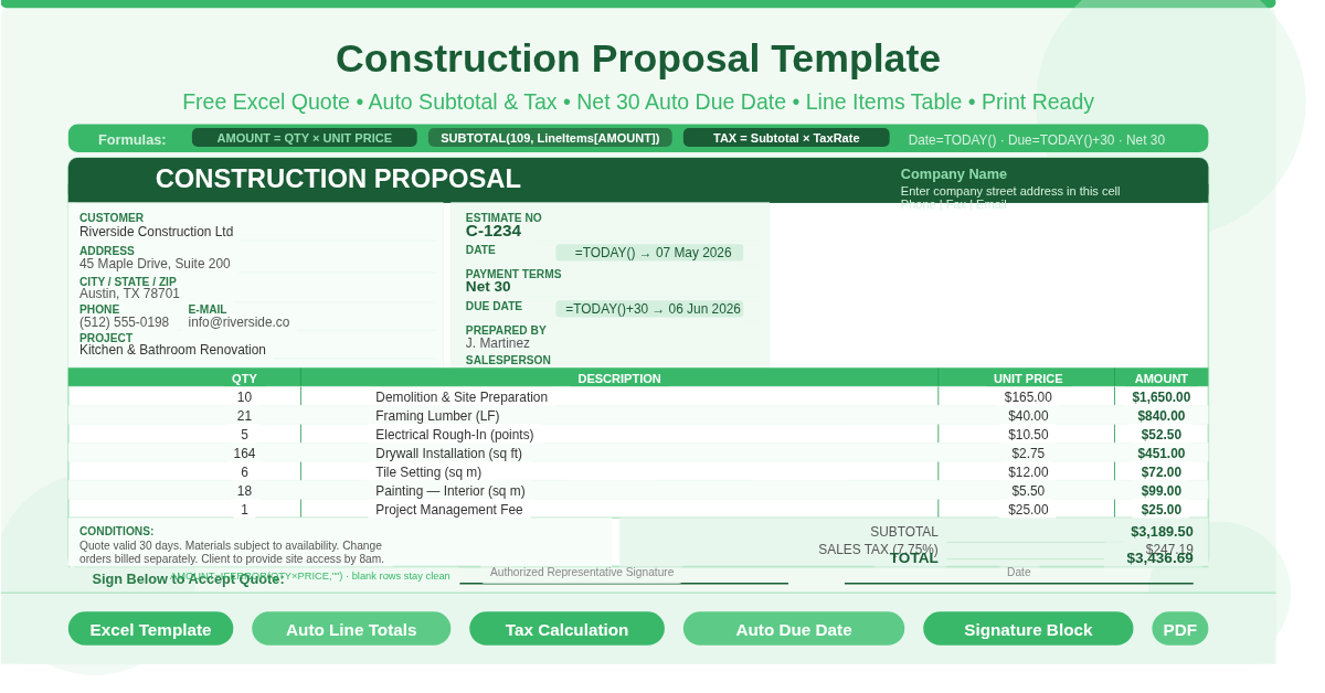
A free Excel construction proposal template that calculates subtotals, tax, and payment due dates automatically — professional, print-ready quotes in minutes.
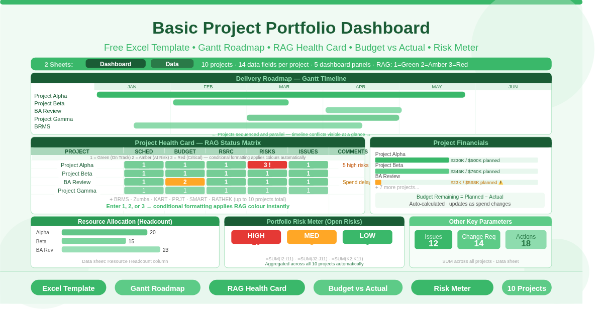
A free Excel project portfolio dashboard that tracks schedule, budget, resources, risks, and issues across all your projects in one consolidated view.

SUBTOTAL handles 11 aggregation types. AGGREGATE handles 19 — and it ignores errors. It does everything SUBTOTAL does, then adds MEDIAN, LARGE, SMALL, PERCENTILE, and QUARTILE to the same filter-aware framework. When a #DIV/0! in one cell breaks your SUBTOTAL total, AGGREGATE skips it. When you need the median of filtered data — which SUBTOTAL cannot compute — AGGREGATE delivers it with a single formula. This guide covers both syntax forms, all 19 function numbers, all 8 option codes, and six practical examples: error-tolerant SUM and AVERAGE, filter-aware MEDIAN and five-number summary, k-th LARGE and SMALL on filtered data, PERCENTILE and IQR outlier bounds, a trimmed mean that removes extreme outliers before averaging, and visible-row RANK. It also explains the most important option choice: use option 5 for most filtered tables, option 7 when data also contains errors, and options 0–3 in grouped reports to prevent grand totals from double-counting group subtotals.
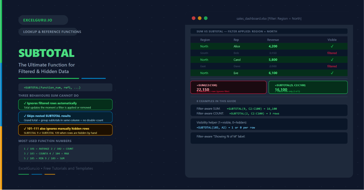
Filter a table and SUM keeps counting every row — including the hidden ones. SUBTOTAL fixes this. It is the only native Excel function that automatically ignores filtered-out rows, updating the moment a filter is applied or removed. This guide covers all 11 aggregation types across both function number ranges (1–11 and 101–111), with eight practical examples: filter-aware SUM, COUNT, AVERAGE, MAX and MIN; group subtotals with a grand total that avoids double-counting; the difference between function 9 and 109 when rows are hidden manually; using SUBTOTAL(103) as a per-row visibility indicator for filter-aware conditional sums; Excel Table Total Row integration; AGGREGATE for median, LARGE, and error-tolerant totals; a live KPI dashboard with a “Showing N of M deals” label; and why SUMIF fails on filtered data — and how to fix it.

A list of 500 numbers tells you almost nothing at a glance. Group them into bins and the shape of the distribution becomes immediately visible — where values cluster, where they thin out, and whether the data skews left or right. The FREQUENCY function performs that grouping in a single formula. This guide covers eight practical examples: building a basic frequency table, charting it as a histogram with gap width set to zero, converting counts to relative frequencies and cumulative percentages, generating dynamic bins with SEQUENCE that update as data changes, counting students per grade band, measuring manufacturing defect rates across tolerance zones, comparing two distributions side-by-side, and using the FREQUENCY distinct-count trick to find unique values. It also covers the key behaviour most analysts miss: FREQUENCY always returns one more value than the number of bin boundaries — that extra row is the overflow bucket, and forgetting it silently drops data.
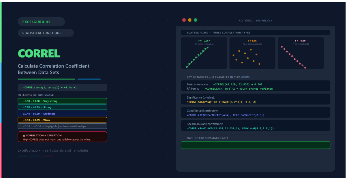
Two columns of numbers — do they move together? The CORREL function answers with a single number between −1 and +1. A result of +0.967 means a very strong positive relationship: when one variable rises, the other rises proportionally. A result of −0.841 means a strong inverse relationship. A result near zero means little or no linear association exists.
This guide covers eight practical examples: basic correlation between two variables, building a 4×4 correlation matrix with conditional formatting, testing statistical significance using the t-test and TDIST, filtering to a specific category with conditional CORREL, rolling correlation to track how the relationship changes over time, finding the strongest pairs across a matrix using LARGE and SMALL, calculating Spearman rank correlation for non-normal or outlier-heavy data, and building a self-updating dashboard that outputs a plain-English label like “r = 0.967 (Very strong positive).” The guide also covers the most important limitation: a high CORREL result does not mean one variable causes the other.

Learn how to use Excel’s LOGEST function for exponential regression. This tutorial covers growth factor extraction, CAGR, R², F-statistic, p-values, exponential decay, half-life, multi-variable models, and 8 practical examples.

Learn how to use Excel’s LINEST function for full linear regression analysis in the given dataset. This blogpost covers slope, intercept, R², F-statistic, p-values, standard errors, multiple regression, polynomial curves, and residual analysis with 8 real world examples.

Excel has no dedicated tick-mark button, but it offers five distinct ways to insert one. The Symbol dialog works for one-off insertions with no setup. Alt+0252 in Wingdings is the fastest keyboard-only method. Shift+P in Wingdings 2 is even quicker once the column is pre-formatted. The CHAR function brings ticks inside formulas — combine it with IF to show a tick when a task is done and a cross when it isn’t. Unicode ✓ and ✔ paste directly into any font without changing a thing. This guide covers all five methods, then shows how to count ticks with COUNTIF, restrict a column to ticks and crosses only using data validation, and color entire rows green or red with conditional formatting

Excel has no built-in SPELLNUMBER function, but three methods fill the gap. The VBA NumToWords function is the most flexible — paste the code once into a module, save as .xlsm, and use =NumToWords(A1) anywhere in the workbook. The AmountToWords extension adds currency and sub-unit names, producing invoice-ready output like “One Thousand Two Hundred Fifty Dollars and Seventy-Five Cents” automatically. For macro-restricted environments, a LAMBDA function defined in the Name Manager achieves the same result with no VBA at all — fully compatible with .xlsx files. This guide covers all three methods with eight practical examples: basic conversion, multi-currency invoice lines (USD, GBP, AED, INR, EUR), cheque format with the XX/100 fraction convention, a dynamic currency table driven by XLOOKUP, and how to lock the output as static text before sharing a finalised document.