
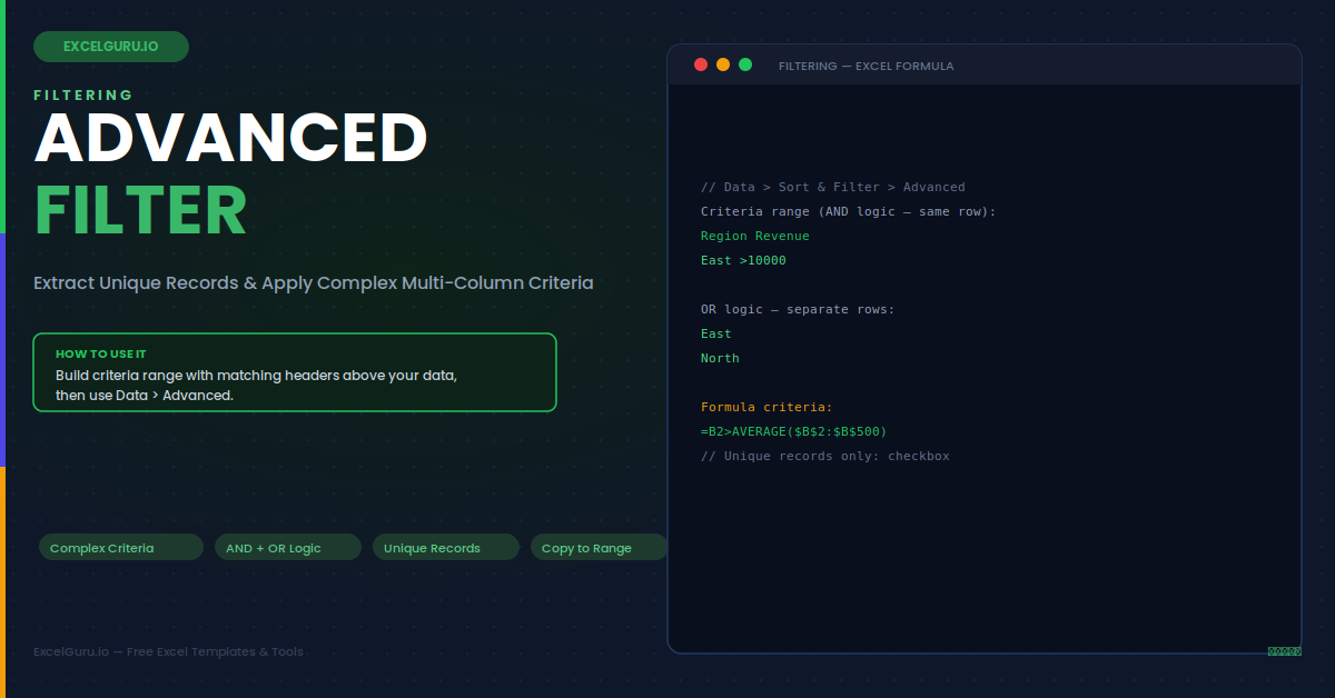
AutoFilter works well for simple single-column filtering. However, it cannot handle complex multi-column criteria, copy results to a different location, or accept formula-based conditions. Excel's Advanced Filter removes all three limitations. It reads criteria from a separate range you build on the sheet, supports any combination of AND and OR logic across any number of columns, copies matching rows to a destination without touching the source data, and accepts any formula returning TRUE or FALSE as a filter criterion. This guide covers the full criteria range syntax, all six key capabilities, and the most common troubleshooting scenarios.
Advanced Filter vs AutoFilter
Both tools filter rows, but they work in fundamentally different ways. Understanding the key differences helps you choose the right tool and avoid confusing the two.
- Filter interface: AutoFilter uses dropdowns in column headers. Advanced Filter uses a separate criteria range you build on the sheet.
- OR logic across different columns: AutoFilter cannot do this. Advanced Filter supports it using separate criteria rows.
- Copy results to another location: AutoFilter filters in place only. Advanced Filter can copy matching rows to a destination, leaving the source untouched.
- Formula-based criteria: AutoFilter does not support this. Advanced Filter accepts any formula returning TRUE or FALSE.
- Duplicate removal in output: AutoFilter has no built-in option. Advanced Filter includes a "Unique records only" checkbox.
Building the Criteria Range
The criteria range is the foundation of every Advanced Filter operation. It consists of a header row followed by one or more criteria rows. The header names must exactly match your data column headers — including capitalisation and spacing. AND logic places two conditions on the same row. OR logic places conditions on separate rows. A blank criteria row means "match everything" and should be avoided.
Example 1: Filter In Place with AND Criteria
Filtering in place is the simplest Advanced Filter use case. Matching rows remain visible in the original table and non-matching rows are hidden — identical to AutoFilter but with richer criteria syntax. This is most useful when you need AND conditions across multiple columns that AutoFilter cannot express from a single dropdown sequence. The filter is cleared with Data > Clear, or by re-running Advanced Filter with an empty criteria range below the header row.
In the criteria range, the header row contains "Region", "Quarter", "Revenue" — exactly matching the data column headers. The criteria row below contains "East", "Q4", ">10000". Advanced Filter consequently shows only rows satisfying all three conditions simultaneously. Adding a second criteria row with "North", "Q4", ">5000" would additionally include matching North rows using OR logic between the two criteria rows.
Example 2: Copy Results to Another Location
Copying to another location is one of Advanced Filter's most powerful capabilities. The source data remains completely untouched — every row stays visible and no rows are hidden. Matching rows are copied to a different area of the sheet or to a different sheet entirely. This is specifically ideal for producing extracts, exception reports, or feeding summary tables from a larger dataset without modifying the original data in any way. The copy operation is static: re-run Advanced Filter whenever the source data changes to refresh the extract.
Example 3: Extract Unique Records
The "Unique records only" checkbox removes duplicate rows from the output without needing UNIQUE, DISTINCT, or any other formula. It works on the full selected row — a row is counted as a duplicate only if every selected column matches another row identically. This is consequently the fastest way to de-duplicate a list in any version of Excel, including Excel 2010 and 2013 where the UNIQUE function does not exist. It also works for multi-column unique combinations by selecting multiple columns in the List range.
Example 4: OR Criteria Across Multiple Columns
AutoFilter cannot express OR conditions across different columns. It applies separate conditions to each column independently, which is AND logic between columns. Advanced Filter handles cross-column OR by using separate criteria rows. Each row represents an independent condition. A data row that matches any one criteria row appears in the output. This makes multi-condition extracts that would require multiple separate AutoFilter steps possible in a single Advanced Filter run.
Example 5: Formula-Based Criteria
Formula criteria are the most powerful Advanced Filter feature. Any formula returning TRUE or FALSE can serve as a criterion — enabling filters that no standard dropdown or value comparison can express. The formula must reference the first data row using a relative row reference (row 2 if headers are in row 1). The header cell above the formula must be blank or a label that does not match any data column header. If it matches a column header, Excel ignores the formula and treats it as a field comparison instead of evaluating it as a formula.
Example 6: Extract Specific Columns in a Custom Order
When copying to another location, you can extract only the columns you need — and in any order you choose. Typing specific column headers in the destination area before running the filter tells Advanced Filter to copy only those columns. Headers must match data column headers exactly, including capitalisation. The sequence of headers in the destination determines the column order in the output, independently of the source column order. This makes Advanced Filter useful for producing presentation-ready extracts with specific column layouts.
Troubleshooting Advanced Filter
Most Advanced Filter problems trace back to the criteria range. Checking the criteria range first resolves the majority of unexpected behaviour quickly.
Advanced Filter returns all rows with no filtering
This almost always means the criteria range contains a blank row below the header. A blank row in the criteria range is interpreted as "match everything" and consequently returns the entire dataset. It can also mean the criteria header names do not exactly match the data column headers — even a single extra space or different capitalisation prevents matching. Fix this by removing any blank rows below the last criterion, and comparing header text character by character against the data headers.
Formula criteria is being ignored
Formula criteria fail for two reasons. First, the header cell above the formula matches a data column header name — Excel interprets it as a field value comparison instead of evaluating the formula. The fix is to use a blank header or a non-matching label like "Criteria". Second, the formula uses an absolute row reference ($B$2) instead of relative (B2). With an absolute reference, the formula evaluates row 2 for every data row rather than evaluating the current row. Always use relative row references in formula criteria.
Copied output shows wrong columns or is missing columns
Advanced Filter reads the column headers placed in the destination area before copying. If a destination header contains a typo, extra space, or capitalisation difference from the source header, that column is skipped. The output column order follows the destination header order exactly — regardless of the order in the source data. To fix this, type destination headers precisely by copying them directly from the data header row rather than typing from memory.
Frequently Asked Questions
- How do I access Advanced Filter in Excel?+Go to the Data tab and click Advanced in the Sort & Filter group. Before opening the dialog, build a criteria range in a blank area of the sheet — a header row with at least one criteria row below it. When the dialog opens, specify the List range (your data), the Criteria range (your criteria table), and optionally a Copy to location. Click OK. Advanced Filter is available in all Excel versions from Excel 2003 through Microsoft 365.
- Can Advanced Filter be used across different sheets?+The criteria range and List range must be on the same sheet as where you open the Advanced Filter dialog. However, the Copy to destination can be on a different sheet — click the Copy to box, then click the destination cell on the other sheet. A common workaround: activate the sheet containing your data, then run Advanced Filter from that sheet with the Copy to destination set to a cell on another sheet.
- Does Advanced Filter update automatically when source data changes?+No. Advanced Filter produces a static snapshot — it does not create a live formula connection. When source data changes, you must re-run Advanced Filter to update the output. For a live, automatically-updating filter, use Excel 365 dynamic array functions: FILTER() for in-place filtering, or FILTER() combined with UNIQUE() for de-duplicated extracts that update automatically whenever source data changes.
- What wildcards does Advanced Filter support?+Advanced Filter supports three wildcards in text criteria. Asterisk (*) matches any sequence of characters of any length. Question mark (?) matches exactly one character. Tilde (~) escapes a literal asterisk or question mark. For example, "S*" matches all text starting with S, "?????" matches text exactly five characters long, and "~*" matches a literal asterisk. Wildcards only apply to text criteria — they do not work in formula-based criteria rows.