
Incorrect data entry in Excel causes problems that are expensive to fix downstream — wrong currency codes in financial models, invalid dates that break DATEDIF formulas, text values in numeric columns that cause VLOOKUP to return errors. Data Validation prevents these problems at the source by controlling exactly what users can type into a cell. It creates dropdown lists, enforces number ranges, validates date boundaries, restricts text length, displays instructional tooltips before entry, and shows custom error messages when invalid data is entered. This guide covers all eight validation types, six practical scenarios including dependent dropdowns and formula-based rules, and every common troubleshooting scenario.
The Eight Validation Types
Each type targets a different kind of input. Choose the type that matches what you want to restrict — using "Custom" for anything that requires a formula-based condition.
Example 1: Dropdown List from an Excel Table — Auto-Expanding
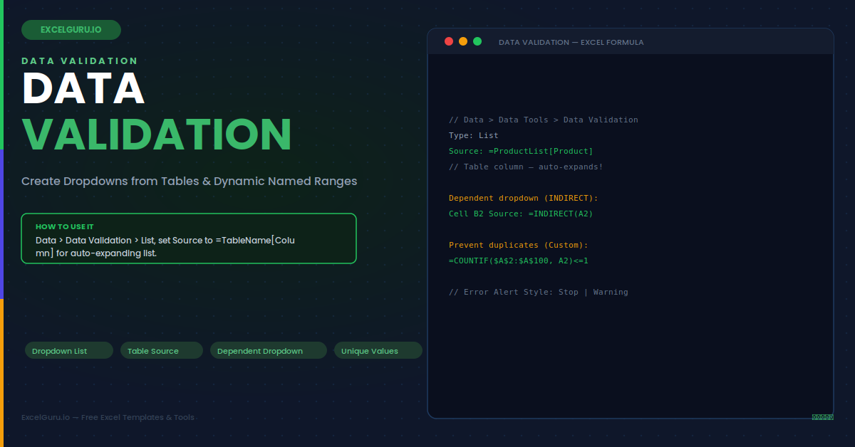
The best practice for dropdown lists is sourcing them from an Excel Table. When the Source references a Table column, the dropdown automatically includes new items added to the Table — the validation Source range does not need updating when the list grows. This makes the dropdown completely maintenance-free. Create your list items in a column, format as a Table (Ctrl+T), name the Table (e.g. "ProductList" in the Table Design tab), then reference it in the Data Validation Source as =ProductList[Product].
=ProductList[Product]. Click OK.Example 2: Dependent Dropdown — Second List Changes Based on First
A dependent dropdown shows different options in the second cell based on what was selected in the first. Selecting "Electronics" in cell B2 changes the Product dropdown in cell C2 to show only electronic products. Selecting "Furniture" changes it to furniture items. This requires creating named ranges for each category — where the range name matches the category text exactly — and using INDIRECT() in the second dropdown's Source field to convert the first cell's value into the corresponding named range.
Example 3: Custom Formula — Enforce Unique Values in a Column
The Custom validation type accepts any formula returning TRUE or FALSE. This enables validation rules that no built-in type can express. For preventing duplicate entries in a column, the formula counts how many times the entered value already exists in the column — if the count is greater than 1, the entry is a duplicate and validation fails. The Error Alert tab controls the message shown when the formula returns FALSE.
Example 4: Input Message — Tooltip Instructions Before Entry
An Input Message is a tooltip that appears whenever the user selects a validated cell — before they type anything. It guides the user on what is expected, reducing the number of Error Alert dialogs triggered by incorrect entries. This is particularly valuable for cells with non-obvious requirements such as specific date formats, reference code patterns, or numeric conventions. The message disappears automatically when the user moves to a different cell and reappears when they return.
Example 5: Error Alert — Custom Message for Invalid Entry
The Error Alert tab controls what happens when a user enters a value that fails the validation rule. Three styles are available. Stop (red X) prevents the entry and requires the user to correct or cancel — use for primary keys, required format fields, and date ranges where invalid entries would cause downstream formula errors. Warning (yellow triangle) shows a message but allows the user to proceed — use for advisory restrictions where occasional exceptions are legitimate. Information (blue circle) shows a note with no enforcement — use for soft reminders only.
Example 6: Date Range Validation — Restrict Entry to Valid Planning Dates
Date validation prevents users from entering past dates in a forward-planning column, dates beyond a project horizon, or weekend dates in a business-days-only field. Use the Date type with "between" and enter the min and max boundaries. Boundaries can be cell references rather than hardcoded values — for example, setting the minimum to =TODAY() enforces a "no past dates" rule that updates daily without anyone editing the validation settings.
Troubleshooting Data Validation
All three issues below are straightforward to diagnose. Each has a specific fix that takes under two minutes to apply.
The dropdown list is empty or shows no items
This typically means the Source range reference is incorrect or points to an empty area. Open Data Validation on the dropdown cell and inspect the Source field. If using a named range, open Name Manager (Ctrl+F3) and verify the range refers to the correct cells with data. If using a Table column reference like =ProductList[Product], verify the Table name matches exactly — Table names are case-sensitive. Also check that the Source range is not on a protected or hidden sheet, which can cause the dropdown to appear empty even when the reference is correct.
The dependent dropdown still shows the previous category's items after changing the parent
The INDIRECT approach does not automatically clear the dependent cell's value when the parent selection changes. The old selection remains, which is now an invalid option for the new parent value. To fix this permanently, add a short VBA Worksheet_Change event macro that clears the dependent cell whenever the parent cell changes: If Target.Address = "$B$2" Then Range("C2").ClearContents. Alternatively, add a note in the Input Message for the parent cell reminding users to clear the dependent cell before selecting a new category.
Pasting values from another source bypasses Data Validation
Data Validation restricts typed entries — it does not block all paste operations. Pasting from an external source (another Excel file, a browser, or a CSV) bypasses validation silently. The pasted value appears in the cell even if it violates the validation rule. To find cells with invalid values after a paste, go to Data > Data Validation > Circle Invalid Data. Excel draws red circles around any cells whose current values violate their validation rules, making it easy to identify and correct them.
Frequently Asked Questions
- How do I create a dropdown list in Excel using Data Validation?+Select the cell or range where you want the dropdown. Go to Data > Data Tools > Data Validation. Set Allow to List. In the Source box, type the items separated by commas ("Open,In Progress,Closed") or select a cell range containing the items ($A$2:$A$10). For an auto-expanding dropdown that updates when the list grows, reference an Excel Table column using =TableName[ColumnName]. Click OK. The dropdown arrow appears in the validated cells — click the arrow to see and select from the list.
- How do I create a dependent dropdown in Excel?+Create named ranges where each name matches exactly one of the parent dropdown options (e.g. a named range called "Electronics" for the electronics products list). Apply a dropdown to the parent cell using the category names as the Source. Apply a second dropdown to the dependent cell using =INDIRECT(ParentCellReference) as the Source. When the user selects a value in the parent dropdown, INDIRECT converts that text value into the matching named range name and the dependent dropdown shows only items from that category.
- Can I use Data Validation to prevent duplicate entries?+Yes. Select the entire column range where duplicates should be prevented (e.g. A2:A100). Open Data Validation and set Allow to Custom. Enter the formula =COUNTIF($A$2:$A$100, A2)<=1 and set the Error Alert style to Stop. When a user types a value that already exists in the range, the COUNTIF returns 2 or more, the formula evaluates to FALSE, and Excel rejects the entry with the custom error message. Note that existing duplicate values already in the range are not removed — only new entries are blocked.
- How do I show a custom error message when Data Validation fails?+Open Data Validation and click the Error Alert tab. Ensure "Show error alert after invalid data is entered" is checked. Choose the style: Stop to reject the entry, Warning to allow it with a confirmation prompt, or Information for a note with no restriction. Enter a Title (shown in bold at the top of the dialog box) and an Error message (shown as the main message text). Click OK. The custom message replaces Excel's default error message text whenever a user enters an invalid value in the validated cell.