
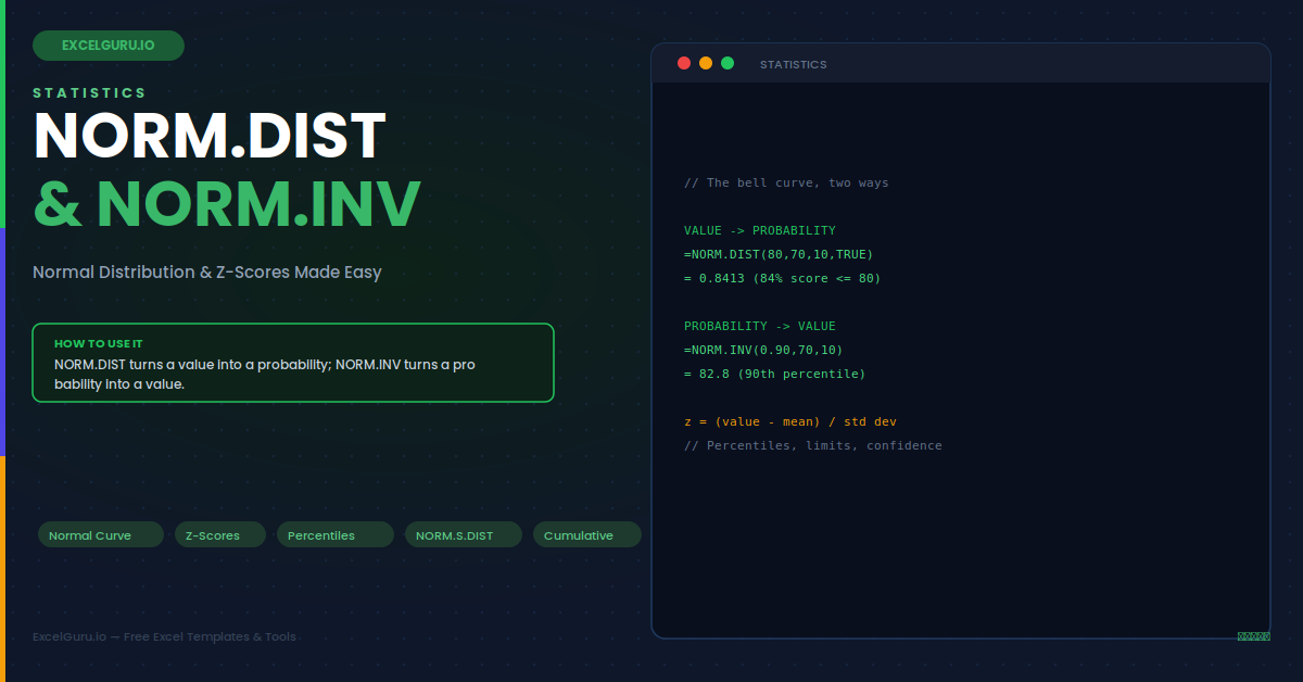
How likely is a value? What score sits at the 90th percentile? Where should a quality cut-off fall? Questions like these come up in finance, manufacturing, grading, and research every day. They all rely on the normal distribution, the famous bell curve. Excel answers them with two paired functions. NORM.DIST turns a value into a probability. NORM.INV does the reverse, turning a probability back into a value. Together they make the bell curve practical.
This guide explains both functions in plain language. First, it covers the bell curve and z-scores. Then it shows exactly when to use each function. Six worked examples and a troubleshooting section make the ideas concrete.
The Bell Curve in Plain Terms
Many real-world measurements cluster around an average. Heights, test scores, and process outputs often follow this pattern. Most values sit near the mean. Fewer values appear as you move outward. Plotted, this forms the familiar bell shape. Two numbers define any normal curve: the mean and the standard deviation. The infographic below shows the curve and the area that NORM.DIST measures.
The mean sits at the centre. Similarly, the standard deviation sets the width. Notably, NORM.DIST measures the shaded area to the left of a value. That area is the probability of getting a value at or below that point.
Z-Scores: A Common Scale
A z-score measures how far a value sits from the mean. Specifically, it counts the distance in standard deviations. For example, a z-score of 1 means one standard deviation above the mean. A z-score of minus 2 means two below. This lets you compare values from different datasets on one scale.
The Syntax of Both Functions
The two functions mirror each other. Essentially, one takes a value and returns a probability. The other takes a probability and returns a value. Knowing which input you have tells you which to use.
Example 1: Probability of a Value or Less
Start with the most common question. What is the chance a value falls at or below a point? NORM.DIST with TRUE answers it directly. This is the shaded area from the infographic.
Example 2: Probability Between Two Values
Often you want the chance of landing in a range. Fortunately, NORM.DIST handles this with a subtraction. You find the area below the upper bound. Then you subtract the area below the lower bound. The difference is the probability between them.
Example 3: Find a Percentile with NORM.INV
Sometimes you know the probability and want the value. That is the job of NORM.INV. For instance, you might need the 90th percentile score. You give NORM.INV the probability 0.90. It returns the matching value.
Example 4: Set a Quality Control Limit
Manufacturing uses these functions constantly. For instance, suppose a process fills bottles. You want the level below which only 1% of bottles fall. That is a lower control limit. NORM.INV finds it from the probability 0.01.
Example 5: Convert a Z-Score to a Probability
When you already have a z-score, use the standard normal functions. NORM.S.DIST takes a z-score directly. It needs no mean or standard deviation. This is handy in statistics work that lives on the z-scale.
Example 6: The Chance of Exceeding a Value
NORM.DIST gives the area to the left. But sometimes you want the area to the right. That is the chance of exceeding a value. Because the total area is 1, you simply subtract from 1. This flips the question around neatly.
Example 7: Estimate a Defect Rate
Quality teams use these functions to predict defects. A part must fall within upper and lower limits. Anything outside counts as a defect. NORM.DIST estimates the fraction outside the limits. This turns a process into a predicted reject rate.
Troubleshooting NORM.DIST and NORM.INV
All three problems below are the most common. Each has a clear cause and a quick fix.
NORM.INV returns a #NUM! error
This error usually means the probability argument is out of range. NORM.INV needs a probability strictly between 0 and 1. A value of exactly 0 or 1 fails, and anything outside that range fails too. Check the first argument carefully. If it came from another cell, make sure that cell holds a proper probability. Percentages are a common trap here. If your value is 90 rather than 0.90, divide it by 100 first. Once the probability sits between 0 and 1, the function works.
The result seems far too small or too large
An answer that looks wrong often traces to the standard deviation argument. People sometimes enter the variance by mistake. Remember that standard deviation is the square root of variance, so the two differ a lot. Confirm you are passing the standard deviation, not the variance. Another common slip is mixing up the mean and standard deviation positions. The order is value, mean, standard deviation. Double-check that each argument is in its correct slot. With the right inputs in the right order, the result falls back into a sensible range.
NORM.DIST returns a tiny height instead of a probability
If NORM.DIST gives a small decimal that is not a probability, you likely set the cumulative argument to FALSE. FALSE returns the height of the curve at the point, not the area beneath it. That height is rarely what you want. For a probability, the shaded area to the left, set the last argument to TRUE. This single change switches the function from curve height to cumulative probability. In almost every practical case, TRUE is the correct choice.
Frequently Asked Questions
- What is the difference between NORM.DIST and NORM.INV?+The two functions are reverses of each other. NORM.DIST takes a value and returns a probability: given a point on the bell curve, it tells you the chance of getting that value or less. NORM.INV takes a probability and returns a value: given a chance like 0.90, it tells you which value sits at that percentile. Use NORM.DIST when you have a number and want its probability, such as the chance a score is below 80. Use NORM.INV when you have a probability and want the matching number, such as the score at the 90th percentile.
- What does the cumulative argument in NORM.DIST do?+The cumulative argument chooses what NORM.DIST returns. Set it to TRUE, and the function gives the cumulative probability, meaning the area under the curve to the left of your value. This is the probability of getting that value or less, and it is what you want in almost every practical situation. Set it to FALSE, and the function returns the height of the bell curve at that exact point, called the probability density. That height is only useful for plotting the curve itself. For any probability question, always use TRUE.
- Why does NORM.INV give a #NUM! error?+NORM.INV requires its probability argument to be strictly between 0 and 1. If you pass exactly 0, exactly 1, or any number outside that range, the function returns a #NUM! error. The most common cause is entering a percentage instead of a decimal: 90 instead of 0.90. Divide any percentage by 100 before passing it in. If the probability comes from another cell, check that the cell holds a valid decimal probability. Once the argument sits properly between 0 and 1, NORM.INV returns the correct value without error.
- How do I find the probability of a value in a range?+Use NORM.DIST twice and subtract. First, find the cumulative probability below the upper bound. Then find the cumulative probability below the lower bound. Subtract the second from the first, and the difference is the probability of landing between the two values. For example, =NORM.DIST(80,70,10,TRUE) - NORM.DIST(60,70,10,TRUE) gives the chance a value falls between 60 and 80. This works because each NORM.DIST call returns the area to the left, so subtracting removes the lower tail and leaves only the middle band you want.