
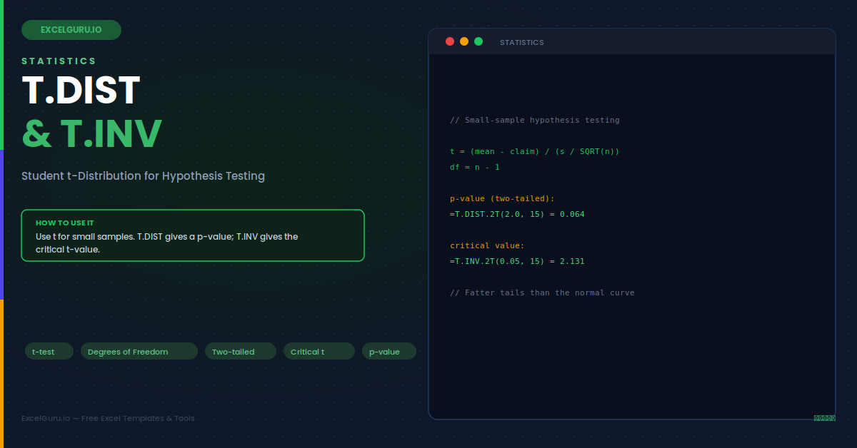
You ran a small experiment. Maybe you tested a new process on twelve samples, or surveyed fifteen customers. Now you need to know if the result is real or just chance. With a small sample, the normal curve is not quite right. It underestimates the uncertainty. The t-distribution fixes this, and Excel gives you two functions for it. T.DIST turns a t-value into a probability. T.INV turns a probability back into a t-value. Together they drive nearly every small-sample hypothesis test.
This guide explains the t-distribution in plain terms. First, it shows why small samples need it. Then it covers each function, including the one-tailed and two-tailed variants. Seven worked examples and a full troubleshooting section follow. By the end, you will be able to run a real t-test in Excel from start to finish. You will also know which function fits each situation.
Why Small Samples Need the t-Distribution
The normal curve assumes you know the true spread of the data. With a small sample, you do not. You only have an estimate. That estimate adds extra uncertainty. The t-distribution accounts for it by making the tails fatter. As a result, extreme values are treated as slightly more likely. This makes the test more cautious. It guards against false confidence from thin data. The infographic below shows the difference.
Notice how the green t-curve sits lower in the middle and higher in the tails. This shape depends on the degrees of freedom. Specifically, degrees of freedom equal the sample size minus one. As the sample grows, the t-curve slowly becomes the normal curve.
The t-Statistic and Degrees of Freedom
Before using these functions, you need two inputs. The first is the t-statistic. It measures how far your sample mean sits from a claimed value. The second is the degrees of freedom. It reflects your sample size. Both feed directly into T.DIST and T.INV.
The Function Variants Explained
Excel offers several t-functions. Each answers a slightly different question. Choosing the right one depends on your test. The table below sorts them out.
| Function | What it returns |
|---|---|
| T.DIST(t, df, TRUE) | Left-tail area up to the t-value (a probability) |
| T.DIST.RT(t, df) | Right-tail area beyond the t-value |
| T.DIST.2T(t, df) | Both tails combined (two-tailed p-value) |
| T.INV(prob, df) | Left-tailed t-value for a given probability |
| T.INV.2T(prob, df) | Two-tailed critical t-value |
Example 1: Find a p-value from a t-Statistic
Start with the most common task. You have a t-statistic and want its p-value. A two-tailed test is typical. So you use T.DIST.2T. The result tells you how surprising your data is.
Example 2: Find a Critical t-Value
Sometimes you want the threshold instead of the p-value. This is the critical t-value. You compare your t-statistic against it. T.INV.2T gives the two-tailed critical value for a chosen confidence level.
Example 3: A Complete One-Sample t-Test
Now put the pieces together. Suppose a supplier claims parts weigh 50 grams. You measure a small sample. You want to test the claim. Here is the full workflow in Excel.
=AVERAGE(range) and the sample standard deviation with =STDEV.S(range).=COUNT(range). Then set df = n minus 1.=(mean-50)/(s/SQRT(n)).=T.DIST.2T(ABS(t), n-1). Compare it to 0.05.Example 4: One-Tailed Test for an Increase
Some questions have a direction. You may only care if a value went up. For instance, did a new method raise output? A drop would not interest you here. That calls for a one-tailed test. It puts all the risk in one tail. Therefore, you use the right-tailed function.
Example 5: Build a Confidence Interval
The t-distribution also builds confidence intervals for small samples. You take the sample mean. Then you add and subtract a margin. That margin uses the critical t-value. This gives a plausible range for the true mean.
Example 6: Compare T.DIST with the Normal Curve
It helps to see how t differs from z. For the same value, the t-distribution gives a larger tail. This reflects the extra uncertainty of a small sample. As degrees of freedom rise, the gap shrinks.
With only 5 degrees of freedom, the t tail is much larger. By 30 degrees of freedom, it is close to the normal value. Consequently, large samples can often use the simpler z approach.
Example 7: A Paired-Difference Test
A paired test compares before and after values on the same subjects. You work with the differences. Then you test whether their average differs from zero. The t-distribution handles this small-sample case well.
Troubleshooting T.DIST and T.INV
All three problems below are the most common. Each has a clear cause and a quick fix.
You get a #NUM! error
This error usually points to an out-of-range argument. T.INV and T.INV.2T need a probability between 0 and 1. A value of 0, 1, or beyond will fail. Check that first argument carefully. The degrees of freedom must also be at least 1. A value below 1 triggers the error too. Another trap is passing a negative t-value to T.DIST.2T or T.DIST.RT, which expect a non-negative input. Wrap the t-value in ABS to be safe. Once the inputs sit in their valid ranges, the error clears.
The p-value seems twice or half what you expected
This almost always means you mixed one-tailed and two-tailed functions. A two-tailed p-value is exactly double the one-tailed value for the same t. So T.DIST.2T returns twice what T.DIST.RT gives. Decide which test you actually need first. Use a two-tailed test when a difference in either direction matters. Use a one-tailed test only when the direction is set in advance. Matching the function to the test removes the factor-of-two confusion at once.
Results differ from an old TDIST formula
Older Excel used a single TDIST function with a tails argument. The newer functions split this into separate names. TDIST(x, df, 2) matches T.DIST.2T(x, df). TDIST(x, df, 1) matches T.DIST.RT(x, df). If you are updating an old workbook, map each call to its modern equivalent carefully. The legacy TDIST still works for compatibility, but the newer functions are clearer. Confirming which version a formula uses explains most differences between old and new sheets.
Frequently Asked Questions
- When should I use the t-distribution instead of the normal distribution?+Use the t-distribution when your sample is small and you do not know the true population standard deviation, which is the usual situation in real testing. Because you estimate the spread from the sample itself, there is extra uncertainty, and the t-distribution accounts for it with fatter tails. As a rough guide, samples under about 30 clearly benefit from the t approach. As the sample size grows, the t-distribution gradually becomes the normal distribution, so for large samples the two give almost identical results and either can be used.
- What is the difference between T.DIST, T.DIST.RT, and T.DIST.2T?+All three work with the t-distribution but return different areas. T.DIST with the cumulative argument TRUE gives the left-tail area up to your t-value. T.DIST.RT gives the right-tail area beyond your t-value, which suits a one-sided test looking for an increase. T.DIST.2T gives the combined area in both tails, which is the two-tailed p-value used when a difference in either direction matters. The two-tailed result is always exactly double the one-tailed result for the same t-value, so choosing the right function depends entirely on the test you are running.
- How do I find a critical t-value for a hypothesis test?+Use T.INV.2T for a two-tailed test or T.INV for a one-tailed test. For a 95% confidence level, the alpha is 0.05, so =T.INV.2T(0.05, df) returns the two-tailed critical value, where df is your degrees of freedom. You then compare the absolute value of your t-statistic against this critical value. If your t-statistic exceeds the critical value, the result is statistically significant and you reject the null hypothesis. If it falls below, the result is not significant. The critical value acts as the threshold your evidence must cross.
- What are degrees of freedom in a t-test?+Degrees of freedom reflect how much independent information your sample contains for estimating variability. For a simple one-sample t-test, the degrees of freedom equal the sample size minus one, because one value is effectively used up when you estimate the mean. So a sample of 16 has 15 degrees of freedom. This number shapes the t-distribution: fewer degrees of freedom produce fatter tails and a more cautious test, while more degrees of freedom produce a curve closer to the normal distribution. You pass the degrees of freedom directly into T.DIST and T.INV as an argument.