
When will this pump fail? Do early failures come from manufacturing faults, or does the part simply wear out with age? Reliability engineers live with these questions, and one distribution answers them all. The Weibull distribution is the workhorse of failure analysis, because a single shape parameter can model early-life failures, random failures, and wear-out failures alike. Excel provides it through WEIBULL.DIST. You supply a time, a shape, and a scale, and it returns the probability of failure by that time.
This guide explains the Weibull distribution in plain terms. First, it shows what the shape and scale parameters do. Then it covers the cumulative switch and the famous bathtub curve. Seven worked examples and a full troubleshooting section follow. By the end, you will forecast failures and read reliability data with confidence.
Why the Weibull Is So Flexible
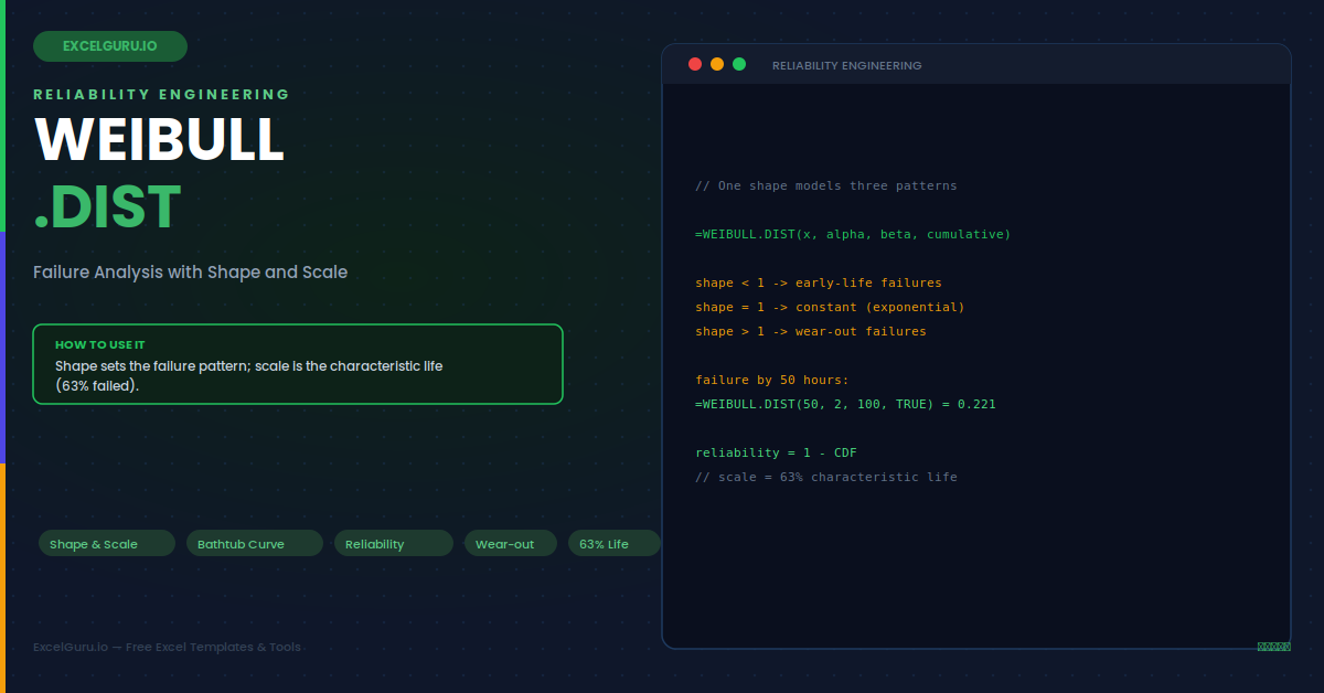
Most distributions model one kind of behaviour. The Weibull models three. Its secret is the shape parameter. Change that one number, and the failure pattern changes completely. No other input is needed to switch modes. The infographic below shows all three regimes at once.
A shape below 1 means early failures dominate, often from defects. A shape of exactly 1 means a constant failure rate, identical to the exponential. A shape above 1 means failures rise with age, the classic wear-out pattern. Consequently, one function covers a product entire life cycle. This is why the Weibull appears everywhere in reliability work. It replaces several narrower models with a single flexible one.
The Two Parameters: Shape and Scale
WEIBULL.DIST relies on two parameters. The shape sets the pattern of failure over time. The scale sets the typical lifetime. Together they define the whole curve. Understanding each one makes the function easy to use.
The Syntax and the Cumulative Switch
WEIBULL.DIST takes four arguments. Two describe the distribution shape. The fourth is the cumulative switch. As with other distributions, that switch changes the meaning.
Example 1: Probability of Failure by a Time
Start with the core reliability question. What is the chance a part has failed by a certain age? You set cumulative to TRUE. This gives the cumulative failure probability. It is the single most-used Weibull calculation.
Example 2: The Reliability (Survival) Value
Reliability is the flip side of failure. What is the chance a part survives past a time? You use the complement rule. Because the total is 1, you subtract the cumulative failure value. This survival figure drives warranty and maintenance decisions.
Example 3: Identify the Failure Pattern
The shape parameter reveals the failure mode. Analysts fit failure data to estimate it. Once known, it guides real decisions. A low shape points to quality problems, while a high shape points to ageing. The table below links each shape to a real-world meaning.
| Shape value | Failure pattern and likely cause |
|---|---|
| Below 1 | Early failures, often defects or poor assembly |
| About 1 | Random failures at a constant rate |
| Above 1 | Wear-out, fatigue, or ageing failures |
Example 4: The Bathtub Curve
The famous bathtub curve combines all three phases. First comes an early period of high, falling failures. Then a long stable period of random failures. Finally a wear-out period of rising failures. The Weibull models each phase with a different shape. This curve underpins most reliability planning.
Example 5: Find the Characteristic Life
The scale parameter has a neat meaning. It is the time by which about 63% of items fail. You can verify this directly in Excel. Set the time equal to the scale and check the result. The answer is always about 63%, whatever the shape.
Example 6: Build a Failure-Probability Table
To see the full picture, list a range of times. You place the times in a column. Then you compute the cumulative failure beside each. This traces how failure risk grows with age.
The failure column uses TRUE for each time. The reliability column is one minus that value. Together they show risk rising and reliability falling as parts age. Plotting these columns gives clear failure and survival curves. Maintenance teams use them to time replacements.
Example 7: Guard the Parameters
Both the shape and scale must be positive. A zero or a negative value has no meaning here. A short guard flags a bad parameter before calculating. This keeps any reliability model tidy and easy to share.
Troubleshooting WEIBULL.DIST
All three problems below are the most common. Each has a clear cause and a quick fix.
You get a #NUM! error
This error means a parameter is out of range. Both the shape alpha and the scale beta must be greater than zero, so a value of zero or below fails at once. The time value x must not be negative either. Check all three against these limits. A common slip is swapping the shape and scale positions in the arguments, which can produce an odd but valid-looking number rather than an error. Confirm each argument sits in its correct slot and within range, and the function returns a proper value.
The result is a density height, not a probability
If WEIBULL.DIST returns a strange value instead of a probability, you likely set cumulative to FALSE. FALSE returns the height of the density curve at that point, which is not a probability and can behave oddly. For the chance of failure by a given time, set cumulative to TRUE, which returns the cumulative probability you almost always want. This is the same trap that appears with other distribution functions. Keep the switch on TRUE for reliability work, and only use FALSE when you specifically need the density curve for a plot.
The shape and scale seem swapped
If your reliability numbers look wrong, the shape and scale may be in the wrong order. The argument order is time, then shape alpha, then scale beta. Because both are just positive numbers, swapping them does not cause an error, only a wrong answer. Remember that shape is usually a small number like 0.8, 1, or 2, while scale is a lifetime like 100 hours. Checking that each value matches its expected magnitude usually reveals a swap. Once shape and scale sit in their correct positions, the failure probabilities return to sensible values.
Frequently Asked Questions
- What does the WEIBULL.DIST function calculate?+Essentially, WEIBULL.DIST calculates failure probabilities for reliability analysis, based on a flexible distribution defined by a shape and a scale parameter. You provide a time or age, the shape alpha, the scale beta, and a cumulative switch. When cumulative is TRUE, it returns the probability that an item has failed by that time; when FALSE, it returns the density curve height. For example, =WEIBULL.DIST(50, 2, 100, TRUE) gives the chance of failure by 50 hours for a wear-out pattern with a 100-hour characteristic life. Its flexibility makes it the standard tool for modelling product lifetimes and failure forecasting.
- What does the shape parameter mean?+Specifically, the shape parameter controls how the failure rate changes over time, which reveals the failure mode. A shape below 1 means the failure rate decreases with age, pointing to early-life failures from defects or poor assembly. A shape of exactly 1 means a constant failure rate, identical to the exponential distribution and typical of random failures. A shape above 1 means the failure rate increases with age, the signature of wear-out, fatigue, or ageing. Because of this, the shape parameter tells you not just when things fail but why, which directly guides whether to improve quality control or schedule preventive replacements.
- What is the characteristic life or scale parameter?+Notably, the scale parameter, often called the characteristic life, is the time by which about 63% of items have failed, regardless of the shape value. If you set the time equal to the scale in WEIBULL.DIST with cumulative TRUE, you always get roughly 0.632. This makes the scale a convenient benchmark for the typical lifetime of a population. A larger scale means a longer-lived product. While the shape tells you the pattern of failures over time, the scale tells you the overall timeframe, so the two together fully describe how and when a population of items fails.
- How is Weibull related to the exponential distribution?+Because the Weibull is a generalisation, the exponential distribution is simply the special case where the shape parameter equals 1. At that shape, the failure rate is constant over time, which is exactly the memoryless behaviour of the exponential. When the shape moves away from 1, the Weibull adds something the exponential cannot: a failure rate that rises or falls with age. This is why the Weibull is preferred for components that wear out, where older parts fail more readily, while the exponential suits truly random failures. In short, if you need a changing failure rate, the Weibull is the more general and appropriate choice.