
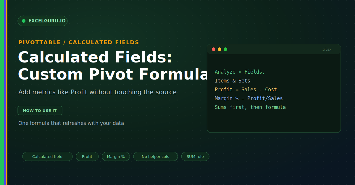
You build a PivotTable and it summarises your data beautifully. Then a manager asks for profit, and your source has only Sales and Cost. The quick fix is to add a helper column in the raw data. However, that clutters the source and breaks when the data refreshes. A calculated field is the clean answer. It adds a new formula-driven field right inside the PivotTable, without touching a single source row.
This guide shows how calculated fields really work. First, it explains what they do and the one rule that trips most people. Then it walks through practical formulas you will actually use. Real examples, limits, and a full troubleshooting section follow. By the end, you will add custom metrics to any PivotTable with confidence.
What a Calculated Field Is
A calculated field is a formula that lives in the PivotTable. It builds a new field from the fields you already have. For example, Profit can come from Sales minus Cost. Notably, the source data never changes. The infographic below shows the idea.
Because the field lives in the pivot, it refreshes with your data. So a new month of sales flows straight through it. You also keep the source clean and simple. As a result, one formula serves every future refresh.
The One Rule That Trips Everyone
Here is the rule that causes most confusion. A calculated field works on the totals, not on each row. In other words, it sums the fields first, then applies your formula. Therefore ratios can surprise you, as the next infographic shows.
Notice the gap between the two results. The simple average of the row prices is 20. Yet the calculated field returns 25, a weighted figure. Both numbers are valid, but they answer different questions. So always check which one your report truly needs.
Calculated Field or Calculated Item
Excel offers two similar tools, and people mix them up. A calculated field adds a new column across the whole pivot. A calculated item adds a new row inside one existing field. Consequently, they solve very different problems.
Most tasks call for a calculated field. You reach for a calculated item only rarely. For instance, you might combine two quarters into one custom item. In general, start with a field and switch only when needed.
How to Create a Calculated Field
The steps are short once you know the menu. You open the Fields, Items and Sets dialog. Then you name the field and type a formula. Finally, Excel drops it into the values area.
Example 1: Profit From Sales and Cost
Start with the classic profit metric. Your source holds Sales and Cost only. A calculated field turns them into Profit at once. Then it totals correctly across every group.
Example 2: Commission at a Fixed Rate
Sales teams often earn a set commission. You can model it with a constant in the formula. Here a rate of ten percent works well. So the pivot shows payable commission by rep.
Example 3: Margin Percent (Mind the Rule)
Margin percent is a favourite metric, but recall the rule. The field divides the summed profit by summed sales. Fortunately, that is exactly right for a margin. So this ratio behaves the way you expect.
Example 4: A Bonus Flag With IF
You can even branch with a simple IF. Suppose a bonus applies above a sales threshold. The formula returns a value only when the total qualifies. Therefore the pivot flags strong performers automatically.
When to Use a Measure Instead
Calculated fields are handy, but they have limits. They cannot count distinct values or average rows properly. For those jobs, a Data Model measure wins. Because DAX runs row by row, it handles them with ease.
Troubleshooting Calculated Fields
All three problems below are the most common. Each has a clear cause and a quick fix.
The result looks wrong for a ratio
This almost always comes back to the totals rule. The field sums each part first, then divides. So a price or rate may look higher or lower than expected. First, decide whether you want a weighted or a simple average. A weighted result is usually right for money, such as blended margin. However, if you need the plain average of row ratios, a calculated field cannot do it. In that case, move the data to the Data Model and write a measure instead.
A function will not work in the formula
Calculated fields accept only a limited set of functions. They cannot use COUNTIF, VLOOKUP, or a worksheet range. So a formula that points at cells will fail. Instead, build the field from other fields and constants. Stick to math and simple functions like IF, SUM, and ROUND. For anything richer, a Data Model measure is the better tool. That path unlocks the full DAX function library.
The field is missing after a rebuild
Sometimes a rebuilt or copied pivot drops the field. This happens when the new pivot uses a different cache. First, confirm you are editing the right PivotTable. Then reopen Fields, Items and Sets to check the field list. If it is gone, simply recreate it, since the formula text is short. To avoid the issue, keep related pivots on one shared source. That way they share a cache and the field travels with them.
Frequently Asked Questions
- What is a PivotTable calculated field?+It is a formula that lives inside the PivotTable. It builds a new field from fields you already have. For example, Profit equals Sales minus Cost. Notably, it never changes your source data.
- Why does my ratio field show the wrong number?+Because a calculated field sums each part first. So Sales divided by Units uses the totals, not each row. That gives a weighted result, not a simple average. For a true row average, use a measure instead.
- Can I use IF or VLOOKUP in a calculated field?+You can use IF, but not VLOOKUP or COUNTIF. Calculated fields accept only fields, constants, and basic functions. Moreover, they cannot point at worksheet cells. For richer logic, write a Data Model measure.
- Where do I create a calculated field?+First, click inside the PivotTable. Then open PivotTable Analyze and Fields, Items and Sets. Finally, choose Calculated Field and enter a name and formula. Click OK to add it.