SUBTOTAL handles 11 aggregation types. AGGREGATE handles 19 — and it ignores errors. It does everything SUBTOTAL does, then adds MEDIAN, LARGE, SMALL, PERCENTILE, QUARTILE, and RANK to the same filter-aware framework. The options argument gives precise control over what to exclude: filtered rows, hidden rows, nested aggregates, errors, or any combination. When a formula fails because of a #DIV/0! in one cell, or because you need the median of filtered data, AGGREGATE is the answer.
This guide covers both syntax forms, all 19 function numbers, all 8 option codes, and six practical examples. You will learn how to compute filter-aware medians and percentiles, extract the k-th largest visible value, handle error-contaminated ranges, and build an outlier-aware average. Each example also shows when AGGREGATE has a distinct advantage over its SUBTOTAL equivalent.
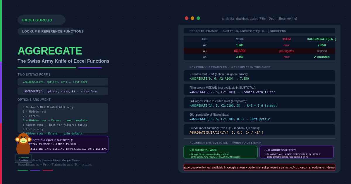
What Makes AGGREGATE Different from SUBTOTAL?
SUBTOTAL ignores filtered and hidden rows, and skips nested SUBTOTAL results. AGGREGATE does all of that and adds two major capabilities. First, it can ignore error values in the data range. A single #DIV/0! or #VALUE! in the range breaks SUBTOTAL — it propagates the error to the result. AGGREGATE skips those cells and computes the result on the remaining valid values. Second, AGGREGATE supports eight additional aggregation functions that SUBTOTAL does not offer.
The options argument is the key that unlocks these capabilities. It is a number from 0 to 7 that specifies exactly which rows to exclude. Options 0–3 control hidden row and error behaviour. Options 4–7 add the ability to ignore nested SUBTOTAL and AGGREGATE results on top of the other exclusions. Choosing the right option is the most important decision when using AGGREGATE.
What Is the AGGREGATE Syntax?
AGGREGATE has two syntax forms. The first (list form) works like SUBTOTAL — pass a range reference and get an aggregate over the entire range. The second (array form) enables LARGE, SMALL, PERCENTILE, and QUARTILE by accepting an array expression with an optional k argument. Always use the array form when the function number requires k.
| Argument | Required? | What it does |
|---|---|---|
| function_num | Required | A number from 1 to 19 specifying the aggregation type. See the full table below. |
| options | Required | A number from 0 to 7 controlling which rows to ignore. This is the key difference from SUBTOTAL. |
| ref1 / array | Required | The data range (list form) or array expression (array form). |
| k | Conditional | Required for LARGE (fn 14), SMALL (fn 15), PERCENTILE.INC (fn 16), QUARTILE.INC (fn 17), PERCENTILE.EXC (fn 18), QUARTILE.EXC (fn 19). Not used for other function numbers. |
What Are the AGGREGATE Function Numbers and Options?
| Fn # | Function | SUBTOTAL equivalent? | Notes |
|---|---|---|---|
| 1 | AVERAGE | Yes (fn 1/101) | — |
| 2 | COUNT | Yes (fn 2/102) | — |
| 3 | COUNTA | Yes (fn 3/103) | — |
| 4 | MAX | Yes (fn 4/104) | — |
| 5 | MIN | Yes (fn 5/105) | — |
| 6 | PRODUCT | Yes (fn 6/106) | — |
| 7 | STDEV.S | Yes (fn 7/107) | Sample std dev |
| 8 | STDEV.P | Yes (fn 8/108) | Population std dev |
| 9 | SUM | Yes (fn 9/109) | — |
| 10 | VAR.S | Yes (fn 10/110) | Sample variance |
| 11 | VAR.P | Yes (fn 11/111) | Population variance |
| 12 | MEDIAN | ✗ AGGREGATE only | — |
| 13 | MODE.SNGL | ✗ AGGREGATE only | Most frequent value |
| 14 | LARGE | ✗ AGGREGATE only | Requires k |
| 15 | SMALL | ✗ AGGREGATE only | Requires k |
| 16 | PERCENTILE.INC | ✗ AGGREGATE only | k = 0 to 1 |
| 17 | QUARTILE.INC | ✗ AGGREGATE only | k = 0 to 4 |
| 18 | PERCENTILE.EXC | ✗ AGGREGATE only | k = 0 to 1 exclusive |
| 19 | QUARTILE.EXC | ✗ AGGREGATE only | k = 1 to 3 |
| Option | Ignores |
|---|---|
| 0 | Nested SUBTOTAL and AGGREGATE functions only |
| 1 | Hidden rows + nested SUBTOTAL/AGGREGATE |
| 2 | Error values + nested SUBTOTAL/AGGREGATE |
| 3 | Hidden rows + error values + nested SUBTOTAL/AGGREGATE |
| 4 | Nothing (no exclusions at all) |
| 5 | Hidden rows only |
| 6 | Error values only |
| 7 | Hidden rows + error values |
Examples 1–4: Core AGGREGATE Patterns
A column that contains formula errors blocks any standard aggregation. IFERROR wrapping on every cell is tedious and can mask genuine problems. AGGREGATE with option 6 or 7 processes valid cells and skips error cells entirely. This is one of AGGREGATE’s most practical advantages over both SUM and SUBTOTAL.
MEDIAN is one of the most requested statistics in filtered tables, and SUBTOTAL cannot produce it. AGGREGATE function number 12 fills this gap. When a filter is applied, AGGREGATE(12, 5, ...) returns the median of visible rows only, updating as the filter changes. This is also the most practical advantage AGGREGATE has over SUBTOTAL in day-to-day analysis.
LARGE and SMALL normally break when errors are present in the range. AGGREGATE with function numbers 14 and 15 handles this cleanly. Specifically, it returns the k-th largest or smallest value from visible, non-error cells only. Specifically, this is useful for top-N reports on filtered tables, where you want the k-th best deal on screen rather than from the full dataset.
Percentile and quartile calculations on filtered data are impossible with standard PERCENTILE.INC or QUARTILE.INC functions, which always consider the full range regardless of filter status. AGGREGATE function numbers 16–19 solve this. They compute percentiles and quartiles from visible rows only, making them the correct tool for distribution reporting on filtered datasets.
Examples 5 and 6: Advanced AGGREGATE Patterns
Outlier-Robust Averages and Rank on Visible Data
A standard average is sensitive to outliers. One extremely high or low value can pull the mean far from the centre of the data. A trimmed mean removes the top and bottom k values before averaging, producing a more robust measure of centre. Building one with AGGREGATE combines LARGE, SMALL, and SUM — working on filtered data and tolerating errors.
The standard RANK function ranks a value against all rows, ignoring filters. Consequently, a filtered row’s rank reflects its position in the full dataset — not among the visible rows. Specifically, combining AGGREGATE LARGE with COUNTIF on the visible range produces a rank for the current filtered view.
Common Issues and How to Fix Them
AGGREGATE returns #VALUE! even with error options
AGGREGATE options 2, 3, 6, and 7 ignore error values — but only in the data cells, not in the arguments themselves. If function_num or options contains an error, AGGREGATE still returns an error. Also check that you are using the correct syntax form. Specifically, LARGE, SMALL, PERCENTILE, and QUARTILE require the array form with four arguments, not three. Calling =AGGREGATE(14, 5, C2:C100) without the k argument returns #VALUE! because k is missing.
The result does not change when I apply a filter
AGGREGATE responds to AutoFilter (Data → Filter or Table filters). Options 1, 3, 5, and 7 ignore hidden rows. However, if Automatic Calculation is off (Formulas → Calculation Options → Manual), AGGREGATE does not recalculate when the filter changes. Press F9 to force recalculation, or switch back to Automatic Calculation. Also confirm that option 5 or 7 is chosen — options 0, 2, 4, and 6 do not exclude hidden rows.
AGGREGATE double-counts grouped subtotals in a grand total
Options 4–7 do not skip nested SUBTOTAL or AGGREGATE results. If a column contains group subtotal rows and a grand total references the entire column, options 4–7 count those subtotal rows as data. Instead, use options 0–3 for grand totals — those automatically skip nested AGGREGATE and SUBTOTAL values.
Frequently Asked Questions
-
What does the AGGREGATE function do?+AGGREGATE performs 19 different aggregation operations — including SUM, AVERAGE, COUNT, MAX, MIN, MEDIAN, LARGE, SMALL, PERCENTILE, and QUARTILE — with the ability to ignore filtered rows, manually hidden rows, error values, and nested SUBTOTAL or AGGREGATE results. It is the extended version of SUBTOTAL, available from Excel 2010 onward. The key advantage over SUBTOTAL is the additional functions (12–19) and the error-tolerance option. The key advantage over SUM and MEDIAN is filter-awareness — AGGREGATE considers only visible rows when the appropriate option is set.
-
What is the difference between AGGREGATE and SUBTOTAL?+SUBTOTAL supports 11 aggregation functions (AVERAGE, COUNT, COUNTA, MAX, MIN, PRODUCT, STDEV, STDEVP, SUM, VAR, VARP). AGGREGATE supports all 11 of those plus 8 more: MEDIAN, MODE, LARGE, SMALL, PERCENTILE.INC, QUARTILE.INC, PERCENTILE.EXC, and QUARTILE.EXC. AGGREGATE also adds an options argument for controlling error handling, which SUBTOTAL does not have. Both work in Excel 2010 and later. SUBTOTAL also works in Google Sheets; AGGREGATE does not. For most filter-aware totals, either works. Use AGGREGATE specifically when you need MEDIAN, LARGE, SMALL, PERCENTILE, or error-tolerant aggregation.
-
Which AGGREGATE option should I use?+For filtered tables where you want filter-aware results, use option 5 (ignore hidden rows). This is the most common choice for everyday dashboards and report totals. If your data also contains formula errors, use option 7 (ignore hidden rows and errors) to handle both simultaneously. In grouped reports with nested AGGREGATE or SUBTOTAL rows, use options 0–3 to prevent double-counting in grand totals. Options 4–7 do not skip nested results. For a clean default that works in most situations, option 5 is the recommended starting point.
More Questions About AGGREGATE
-
Can AGGREGATE replace IFERROR?+For aggregation purposes, yes. Instead of wrapping every cell with IFERROR, use AGGREGATE with option 6 or 7 to ignore errors. For example, =AGGREGATE(9, 6, A2:A100) sums the range and skips any error cells, returning the total of the valid values. This is cleaner and more efficient than =SUMPRODUCT(IFERROR(A2:A100, 0)). However, AGGREGATE only works for the 19 supported aggregation types. If you need a non-aggregation formula to handle an individual error, IFERROR or ISNUMBER+IF is still the right approach.
-
How do I use AGGREGATE for LARGE on filtered data?+Use function_num 14 with option 5 and provide k as the fourth argument: =AGGREGATE(14, 5, C2:C100, 1) for the largest visible value, =AGGREGATE(14, 5, C2:C100, 2) for the second largest, and so on. This is the array form of AGGREGATE — the k argument appears after the range. It returns the k-th largest value from currently visible rows, skipping error cells if option 6 or 7 is set. For a dynamic top-3 table, enter in D2 with ROW()-ROW($D$2)+1 as k and copy down three rows.
-
Does AGGREGATE work with Excel Tables?+Yes. AGGREGATE works with structured table references just like SUBTOTAL. Reference the column using the table column notation: =AGGREGATE(9, 5, SalesData[Revenue]) for a filter-aware SUM of the Revenue column. The Total Row uses SUBTOTAL by default, but you can replace those formulas with AGGREGATE to gain MEDIAN, LARGE, or error-tolerance. Additionally, when new rows are added, the AGGREGATE range expands automatically via the structured reference.