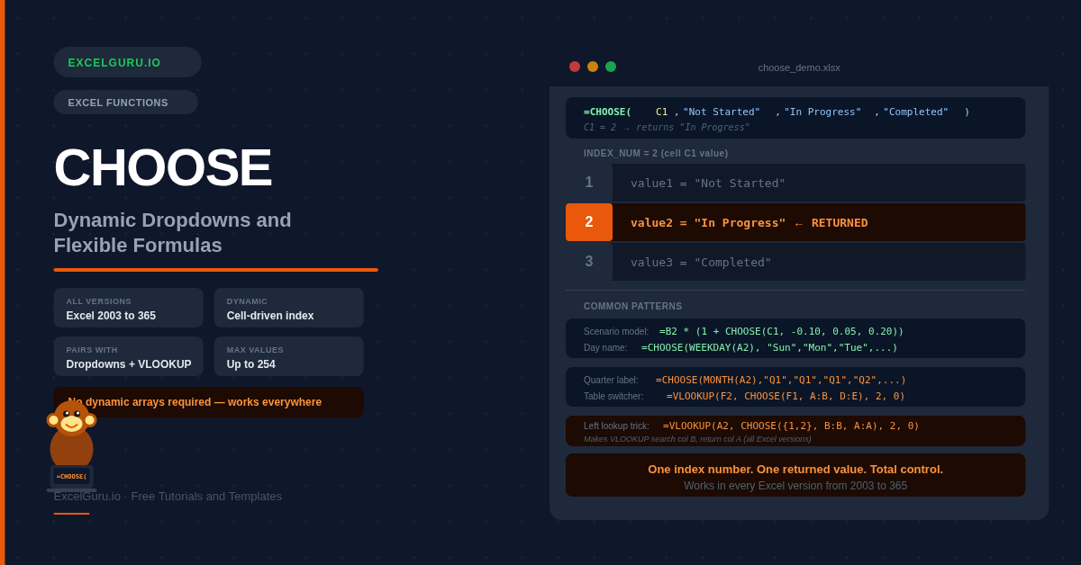
The CHOOSE function is one of Excel's most underused tools. It picks one value from a list based on a number you supply — and because that number can come from a cell, a formula, or a dropdown, the result changes dynamically whenever the number changes. CHOOSE works in every Excel version from Excel 2003 through Microsoft 365, requires no dynamic array support, and is the cleanest way to create scenario selectors, day-name lookups, commission calculators, and dropdown-driven dashboards without nesting a stack of IF statements. This guide covers the full syntax and six practical examples.
CHOOSE Function Syntax
| Argument | Required? | What it means |
|---|---|---|
| index_num | Required | A number from 1 to 254 that picks which value to return. Usually a cell reference so the formula becomes dynamic. Must be a whole number — decimals are truncated. Returns #VALUE! if less than 1 or greater than the number of values provided. |
| value1 | Required | The value returned when index_num = 1. Can be text, a number, a cell reference, a range, or another formula. |
| value2, value3... | Optional | Additional values for index_num 2, 3, and so on. Up to 254 values total. Each can be a different data type — you can mix text, numbers, ranges, and formulas freely. |
The logic is simple: CHOOSE reads the index_num, counts that far into the value list, and returns whatever is in that position. Index 1 returns value1, index 2 returns value2, and so on.
Example 1: Return a Text Label from a Number Code
The most straightforward use — translate a numeric status code or rating into a readable label. Point a dropdown or data entry cell at CHOOSE and it becomes a live label generator.
Example 2: Day Name from a Date
Excel's WEEKDAY function returns 1–7 for each day of the week. Feed that directly into CHOOSE as the index_num to convert any date into a full day name — without complex TEXT formatting or lookup tables.
Example 3: Scenario Selector — Switch Between Calculations
CHOOSE is perfect for building interactive what-if models. Store the scenario number in a single cell (often with a dropdown), then use CHOOSE to pick the multiplier or rate for each scenario. The entire model recalculates instantly when the user changes the selector.
Example 4: CHOOSE as a VLOOKUP Table Switcher
CHOOSE's values can be ranges — not just text or numbers. This makes it possible to pass CHOOSE directly as the table_array argument of VLOOKUP or as an array to other functions. The result is a dynamic lookup that searches a different table based on a user's selection.
=CHOOSE({1,2}, B:B, A:A) creates a virtual two-column table where B is column 1 and A is column 2 — letting VLOOKUP search column B and return column A. This is a well-known workaround that works in all Excel versions.
Example 5: Month Name and Quarter Label
CHOOSE pairs naturally with date functions — use MONTH() to extract a 1–12 month number and feed it directly to CHOOSE. The same pattern returns quarter labels, half-year tags, or any custom period grouping from a date column.
Example 6: Commission Rate Based on Performance Tier
CHOOSE can calculate values, not just return static labels. Use a Boolean expression — one that adds up TRUE/FALSE comparisons — as the index_num to map a number into a tier automatically. This replaces nested IF statements with a single flat formula.
Troubleshooting CHOOSE Errors
#VALUE! error
The index_num is less than 1, greater than the number of values provided, or is text rather than a number. Check the cell referenced as index_num — it must contain a whole number between 1 and the count of your values. If a dropdown or formula feeds this cell, confirm it is returning a number and not text.
Formula returns the wrong value
CHOOSE truncates decimals — 2.9 becomes 2. If a formula produces a decimal index_num, use ROUND() or INT() to convert it to the integer you intend before passing it to CHOOSE.
CHOOSE returns a range but the outer formula errors
When CHOOSE returns a range (for use inside VLOOKUP, MATCH, etc.), some functions require specific range formats. Ensure the ranges passed as CHOOSE values are the same shape and that the outer function accepts an array argument in that position.
Frequently Asked Questions
-
What does the CHOOSE function do in Excel?+CHOOSE returns one value from a list based on an index number you provide. If you give it index 1 it returns the first value, index 2 the second, and so on. The index_num is usually a cell reference so the result changes dynamically when the cell value changes. Values in the list can be text, numbers, cell references, ranges, or other formulas.
-
What is the difference between CHOOSE and IFS?+IFS evaluates independent logical tests — each condition can be a different expression. CHOOSE selects from a fixed list by position number — all conditions share the same index. Use CHOOSE when you already have a numeric code or can generate one with a formula. Use IFS when each condition is a different type of comparison. CHOOSE is also available in all Excel versions while IFS requires Excel 2019 or later.
-
Which Excel versions support CHOOSE?+CHOOSE works in every version of Excel — from Excel 2003 through Microsoft 365. It does not require dynamic array support, making it one of the most universally compatible functions in Excel. This is a key reason to prefer CHOOSE over newer alternatives when building workbooks shared with users on older Excel versions.
-
Can CHOOSE return a range instead of a single value?+Yes. Each value argument in CHOOSE can be a cell range rather than a single value. This is most commonly used to pass a dynamically selected range to VLOOKUP as the table_array argument — letting VLOOKUP search different tables based on the index. It can also create a virtual two-column array using =CHOOSE({1,2}, col_B, col_A) to enable left-lookup with VLOOKUP.
-
How do I use CHOOSE with a dropdown list?+Set the index_num argument to reference the cell containing the dropdown. Create a Data Validation dropdown in that cell with allowed values 1, 2, 3 (and so on). When the user picks a number from the dropdown, CHOOSE immediately returns the corresponding value. For a more user-friendly approach, create the dropdown with text labels and use MATCH to convert the selected label to a position number for CHOOSE.
-
What is the CHOOSE({1,2}, ...) trick for left lookup?+Normally VLOOKUP can only return values from columns to the right of the search column. =CHOOSE({1,2}, col_B, col_A) creates a virtual two-column array where column B becomes the first column and column A becomes the second. Passing this to VLOOKUP lets it search column B and return column A — effectively a left lookup. This is a classic technique that works in all Excel versions, though XLOOKUP and INDEX MATCH are cleaner alternatives in Excel 365 and 2021.