
The same Excel workbook often needs to serve different audiences at different times. A manager needs a high-level summary with sensitive salary columns hidden. An analyst needs the full detail at 80% zoom with frozen panes. The monthly print run needs a specific print area and landscape orientation. Custom Views saves named snapshots of your display and print settings, then restores the complete configuration in one click. No manual reconfiguration. No separate files. This guide covers everything the feature saves, six real-world scenarios, every limitation, and all common troubleshooting steps.
What Custom Views Saves — and What It Does Not
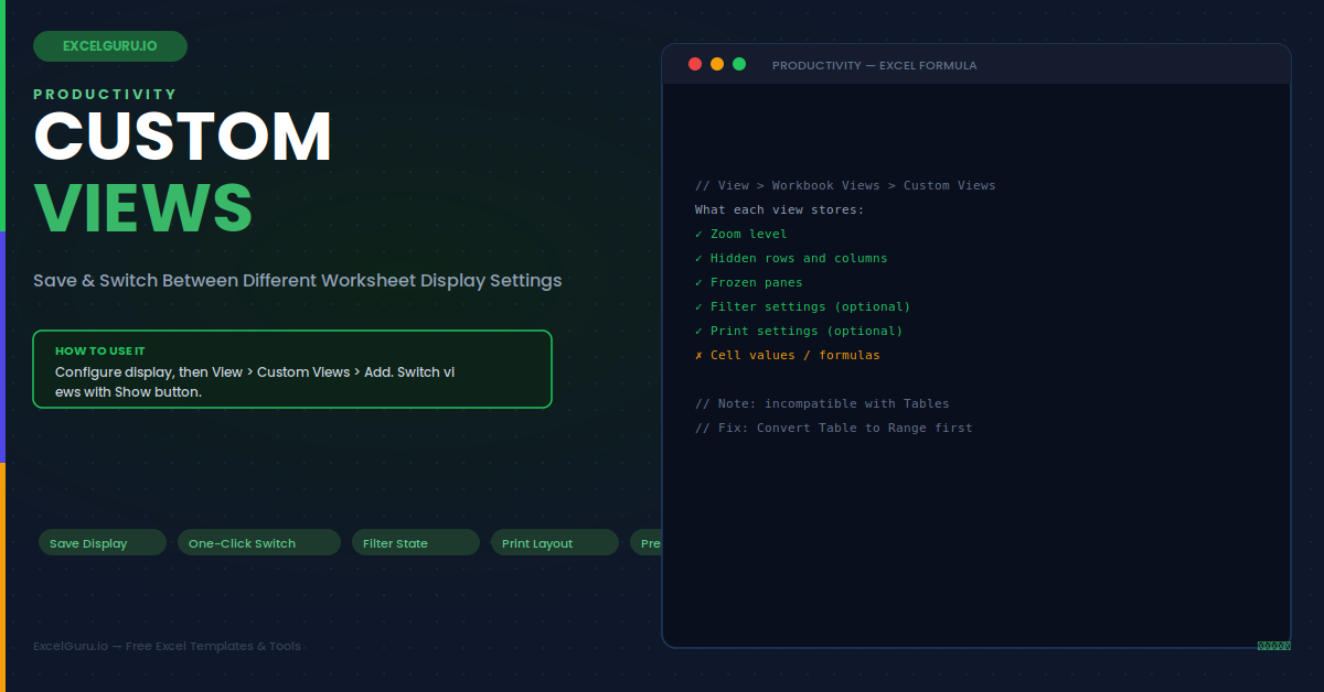
The feature saves display configuration only. It never affects cell values, formulas, or cell formatting. Each setting below is saved per-view and restored when you switch to that view.
Critical Limitation — Excel Tables Disable Custom Views
If any Excel Table (Insert > Table or Ctrl+T) exists anywhere in the workbook, Custom Views becomes completely unavailable. The option is greyed out in the View menu with no error message. To re-enable it, right-click any Table cell and choose Table > Convert to Range. Repeat for every Table across every sheet. Converting preserves all data and formatting but removes auto-expansion, structured references, and filter dropdowns from the Table. Once all Tables are converted, Custom Views becomes available again.
Creating and Switching Views — Step by Step
Configure the display settings you want to save first. The view captures the current state of these settings at the moment you click Add — not a future state.
Example 1: Operations vs Management — Two Views on One Sheet
A financial workbook contains 200 rows of transaction detail and a 15-row summary section at the top. Operations needs all 200 rows at 80% zoom with frozen panes. Management needs only the 15-row summary, all detail rows hidden, at 120% zoom, with the print area set to just the summary section. Both audiences use the same workbook — no version control or audit trail problems from maintaining two files. Switch to the correct view before each screen share or print run.
Example 2: Audience-Specific Columns — Hide Sensitive Data per Role
A payroll workbook has columns for name, department, gross salary, tax deductions, net pay, and employer contributions. The finance team needs all columns. The line manager view shows only name, department, and net pay — all financial columns are hidden. Creating separate named views for each audience means switching takes one click rather than manually hiding and unhiding columns every time. Each view captures exactly which columns are hidden, so restoration is precise and repeatable.
Example 3: Pre-Configured Print Layouts — One View per Format
A monthly report workbook needs three different print formats: an A4 portrait summary for the board pack, a landscape full-detail print for the operations archive, and a landscape combined view for the projector. Each print configuration — print area, orientation, paper size, margins, scaling, header text — takes several minutes to configure manually. Saving each as a Custom View with print settings enabled reduces the monthly print preparation from 15 minutes to under one minute. Switch to the correct view, press Ctrl+P, and the right configuration applies automatically.
Example 4: Saved Filter States — Toggle Between Data Subsets
An analyst regularly switches between three data subsets on the same sheet: all data unfiltered, East region Q4 only, and top-revenue accounts across all regions. Setting up each AutoFilter combination takes 30–60 seconds. Saving each as a Custom View with "Hidden rows, columns and filter settings" checked reduces this to a single click. The saved view restores the exact filter state — which columns are filtered and which values are selected — without the analyst needing to remember or reconfigure anything each time.
Example 5: Presentation Mode — Clean Display for Screen Sharing
During client presentations, the Excel interface shows distracting elements — gridlines, row and column headers, the formula bar. A presentation view hides all of these via View > Show, increases zoom to 150%, and hides all rows and columns not relevant to the current topic. Saving this as "Presentation Mode" means one click transforms the working spreadsheet into a clean, professional display. After the call, one click on "Working View" restores the full interface. The toggle takes under two seconds either way.
Example 6: Renaming and Deleting Views — Maintenance Best Practices
Custom Views cannot be renamed directly after creation — there is no rename option in the dialog. The workaround is straightforward: switch to the view you want to rename, create a new view with the correct name capturing the same settings, then delete the old view. Always create the replacement first before deleting the original. The Custom Views dialog also serves as an audit list — opening it shows all views saved in the workbook. Review and clean up outdated configurations in shared workbooks to prevent confusion about which view applies to which purpose.
Troubleshooting Custom Views
Custom Views problems almost always have one of three causes. Checking these in order resolves the majority of issues.
Custom Views is greyed out in the View menu
An Excel Table anywhere in the workbook disables Custom Views completely. Go to each sheet, click inside any Table, and choose Table Design > Tools > Convert to Range. Repeat for every Table across all sheets in the workbook. After converting all Tables to plain ranges, Custom Views becomes available in the View menu. This is a hard Excel limitation — there is no workaround other than removing all Tables. If Tables are required for other functionality, consider keeping Custom Views and Tables in separate workbooks.
Switching views does not restore the expected filter state
The filter was not saved when the view was originally created. Open Custom Views, delete the view in question, reapply the exact filter configuration you want to preserve, then re-add the view with the "Hidden rows, columns and filter settings" checkbox enabled before clicking OK. Also verify the filter is applied to the same column it was on when you created the original view — filter states are column-position-specific, not column-name-specific. A column inserted between the original creation and the re-creation can shift filter positions.
Print settings are not restored when switching to a print view
Print settings are only saved in a Custom View when the "Print settings" checkbox is enabled at creation time. If the view was created without this checkbox, it captures display settings but ignores page setup entirely. Delete the view, configure all print settings exactly as required — print area, orientation, scaling, margins — then re-add the view with "Print settings" checked. Switching to the view afterwards restores both display and page setup simultaneously, applying the complete print configuration in one click.
Frequently Asked Questions
- What does Excel Custom Views save?+Custom Views save display and print configuration. They always save zoom level, hidden rows and columns, frozen panes, column widths, and row heights. They optionally save AutoFilter state (when "Hidden rows, columns and filter settings" is checked at creation) and full print page setup including print area, orientation, margins, scaling, and headers/footers (when "Print settings" is checked). They do not save cell values, formulas, number formats, font styles, fill colours, chart positions, or PivotTable configurations — only the display and print state of the worksheet.
- Why is Custom Views greyed out in my workbook?+Custom Views is disabled whenever any Excel Table exists in the workbook — even on a different sheet. To re-enable it, right-click any cell inside each Table and choose Table > Convert to Range. Repeat for every Table on every sheet. After all Tables are converted, Custom Views becomes available. This is a hard limitation in Excel with no workaround other than removing all Tables. Converting a Table to a range preserves data and formatting but removes auto-expansion, structured formula references, and filter dropdowns from the Table.
- Can I rename a Custom View after creating it?+Custom Views cannot be renamed directly — there is no rename option in the dialog. The workaround is to switch to the view, create a new view with the correct name using the same settings, then delete the old view. Always create the replacement before deleting the original so you do not lose the configuration. Custom View names are stored inside the workbook file and travel with the file when it is shared — any collaborator who opens the file will see all saved Custom Views in the View menu.
- Do Custom Views work in Excel for Mac and Excel Online?+Custom Views are fully supported in Excel for Mac and work identically to the Windows version, including the Table limitation. They are not available in Excel Online — the browser version does not include the Custom Views option in the View menu. Views created in the desktop Excel application are stored in the workbook file and remain there when opened online, but they cannot be activated, created, or managed from the browser. Use the Excel desktop application for workbooks that depend on Custom Views for their audience-switching workflow.