Concatenating a number with text strips its formatting instantly. You write "Revenue: " & A2 and instead of "Revenue: $48,500.00" you get "Revenue: 48500". The DOLLAR function solves this specific problem. It converts a number to a currency text string with the symbol, thousands separators, and fixed decimal places. Concatenation then preserves the display you want.
Furthermore, DOLLAR rounds its output to the decimal precision you specify. Negative decimal values round to the left of the decimal point. This is useful for executive summaries where whole thousands are clearer than exact cents. This guide covers the full syntax, when to use DOLLAR versus cell formatting versus TEXT, and eight practical examples.
What Is the DOLLAR Syntax?
DOLLAR takes two arguments — the number to format and an optional decimal precision.
| Argument | Required? | What it does |
|---|---|---|
| number | Required | The number to convert to a currency text string. Can be a cell reference, a hardcoded number, or a formula that returns a number. |
| decimals | Optional | The number of digits to the right of the decimal point. Defaults to 2. If positive, rounds to that many decimal places. If zero, shows no decimal point. If negative, rounds to the left of the decimal point — for example, -3 rounds to the nearest thousand. |
How Does the Decimals Argument Work?
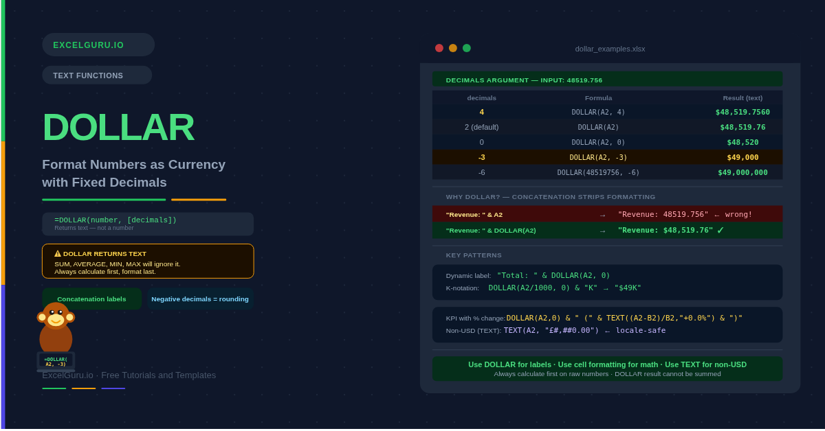
The decimals argument gives DOLLAR its rounding power. Positive values control decimal places. Zero removes the decimal point entirely. Negative values round to the left of the decimal — rounding to tens, hundreds, or thousands. This table shows the full range of effects.
| Decimals | Formula (input: 48519.756) | Result |
|---|---|---|
| 4 | =DOLLAR(48519.756, 4) | $48,519.7560 |
| 3 | =DOLLAR(48519.756, 3) | $48,519.756 |
| 2 (default) | =DOLLAR(48519.756) | $48,519.76 |
| 1 | =DOLLAR(48519.756, 1) | $48,519.8 |
| 0 | =DOLLAR(48519.756, 0) | $48,520 |
| -1 | =DOLLAR(48519.756, -1) | $48,520 |
| -2 | =DOLLAR(48519.756, -2) | $48,500 |
| -3 | =DOLLAR(48519.756, -3) | $49,000 |
| -4 | =DOLLAR(48519.756, -4) | $50,000 |
DOLLAR vs Cell Formatting vs TEXT — Which Should You Use?
Three approaches format a number as currency in Excel. Choosing the right one prevents errors and keeps your workbook maintainable. The key distinction is whether you need the result to remain a number or become text.
| Method | Result type | Works in SUM/AVERAGE? | Best for |
|---|---|---|---|
| Cell formatting (Ctrl+1) | Remains a number | ✅ Yes — the cell is still a number | Display formatting only. Use for all columns that will be summed or averaged. This is the default choice for numeric data. |
| TEXT function | Text string | ❌ No — result is text | Embedding a formatted number inside a sentence when you need full control over the format code. TEXT supports any currency symbol and any custom format string. |
| DOLLAR function | Text string | ❌ No — result is text | Embedding a formatted dollar-symbol value inside concatenated text when a quick currency format is needed. Simpler to write than TEXT for USD with standard commas. |
Examples 1–4: Core Formatting Patterns
The most common use is simply converting a numeric value to a formatted currency string with two decimal places — the standard representation for most currencies. DOLLAR handles the symbol, comma separator, and decimal alignment automatically.
Setting decimals to 0 rounds to the nearest whole dollar and removes the decimal point entirely. This is useful for price lists, invoice totals, and any context where showing cents clutters the display.
Negative decimals round to the left of the decimal point. This is specifically useful for executive-level reports where exact amounts distract from the message. Rounding £48,519,756 annual revenue to the nearest million produces "£49,000,000". That is cleaner at a glance in a presentation or email summary than the precise figure.
This is DOLLAR's primary use case. Joining a number to text with the ampersand operator strips all formatting. The dollar sign, commas, and decimal places all disappear. DOLLAR preserves them. Consequently, reports, email subjects, and summary labels display the number exactly as intended.
Examples 5–8: Advanced Patterns
Dynamic Precision and Conditional Formatting
The decimals argument accepts a cell reference, not just a hardcoded number. This lets users change the display precision by editing a single control cell. It is useful for reports that switch between showing cents and whole dollars depending on the audience.
Nesting DOLLAR inside IF creates formatted currency labels that change based on a condition. This produces self-describing status lines — for example, showing "On target: $48,520" or "Shortfall: $3,480" depending on whether the actual value meets the target, without any manual updating.
DOLLAR uses the system's default currency symbol. On a US-locale machine it outputs a dollar sign ($). On a UK-locale machine it outputs a pound sign (£). Consequently, if you need to embed a specific currency symbol regardless of locale — or a different symbol than the system default — TEXT is the correct function to use instead.
Dashboard cells often need to combine a currency figure with a percentage change, a date, or a comparison label — all in a single self-updating cell. DOLLAR handles the currency part, while TEXT handles other formatted values. Together they produce polished summary labels that update automatically as data changes.
Common DOLLAR Issues and How to Fix Them
SUM returns zero on DOLLAR-formatted cells
DOLLAR returns text, and SUM ignores text values — returning zero or treating the cells as blank. Never apply DOLLAR to cells that will be used in calculations. Keep raw numbers in one column, apply DOLLAR in a separate display column. Calculations always use the raw number column. Consequently, the fix is to restructure the data rather than wrap DOLLAR's output in VALUE.
Currency symbol is wrong — showing $ instead of £
DOLLAR applies the currency symbol based on the system's regional language settings. On a US-locale machine it shows $. On a UK-locale machine it shows £. This is by design. To force a specific symbol regardless of locale, use TEXT instead of DOLLAR: =TEXT(A2, "£#,##0.00") always outputs £ on any machine.
#VALUE! error in DOLLAR
DOLLAR returns #VALUE! when the number argument is text rather than a number, or when the decimals argument contains text instead of a numeric value. Check the source cell with =ISNUMBER(A2) — if it returns FALSE, the cell holds text-formatted numbers. Use VALUE(A2) or apply CLEAN and TRIM to the source cell first, then pass the result to DOLLAR.
Frequently Asked Questions
-
What does the DOLLAR function do in Excel?+DOLLAR converts a number to a text string formatted as currency. It applies the system's default currency symbol, adds thousands separators (commas), and rounds the number to a specified number of decimal places. The default is two decimal places. For example, =DOLLAR(48519.756) returns the text string "$48,519.76". The result is always text — not a number — which makes it ideal for embedding formatted currency values inside concatenated labels and sentences.
-
Why does SUM return zero when I use DOLLAR?+DOLLAR returns a text string, and SUM ignores text values, returning zero. This is the most common DOLLAR mistake. The fix is to keep raw numbers in a source column and use DOLLAR only in a separate display column. All calculations — SUM, AVERAGE, IF comparisons — must reference the source column, not the DOLLAR column. Think of DOLLAR as a label generator, not a number formatter.
-
What is the difference between DOLLAR and TEXT for currency formatting?+Both functions convert a number to a formatted text string. The key difference is control over the currency symbol. DOLLAR always uses the system's default currency symbol — which changes based on the machine's regional settings. TEXT lets you specify any symbol explicitly in the format string — for example, =TEXT(A2, "£#,##0.00") always outputs £ regardless of locale. Use TEXT when the workbook will be used on machines with different regional settings, or when you need a non-default currency symbol.
More Questions About DOLLAR
-
How do I round to the nearest thousand with DOLLAR?+Set the decimals argument to -3. For example, =DOLLAR(48519.756, -3) returns "$49,000". The negative decimals argument rounds to the left of the decimal point — -1 rounds to the nearest ten, -2 to the nearest hundred, -3 to the nearest thousand, and so on. This is useful for executive dashboards where exact cent values distract from the big picture.
-
Can I use DOLLAR to format numbers as £ or €?+DOLLAR cannot specify a currency symbol directly — it always uses the system default. On a UK-locale machine DOLLAR outputs £, and on a US-locale machine it outputs $. To force a specific symbol on any machine, use TEXT: =TEXT(A2, "£#,##0.00") for British pounds, =TEXT(A2, "€#,##0.00") for euros, =TEXT(A2, "¥#,##0") for Japanese yen. The TEXT function accepts any character in the format string, giving you full control over the symbol.
-
Why does my concatenated number lose its currency formatting?+Joining a number to text with the ampersand operator strips all cell formatting — the currency symbol, commas, and decimal places all disappear. This happens because the ampersand works with the underlying numeric value, not the displayed format. Wrapping the number in DOLLAR fixes this: ="Revenue: " & DOLLAR(A2) preserves the symbol and commas and produces "Revenue: $48,519.76" instead of "Revenue: 48519.756". This is the most common reason to use DOLLAR rather than cell formatting.