
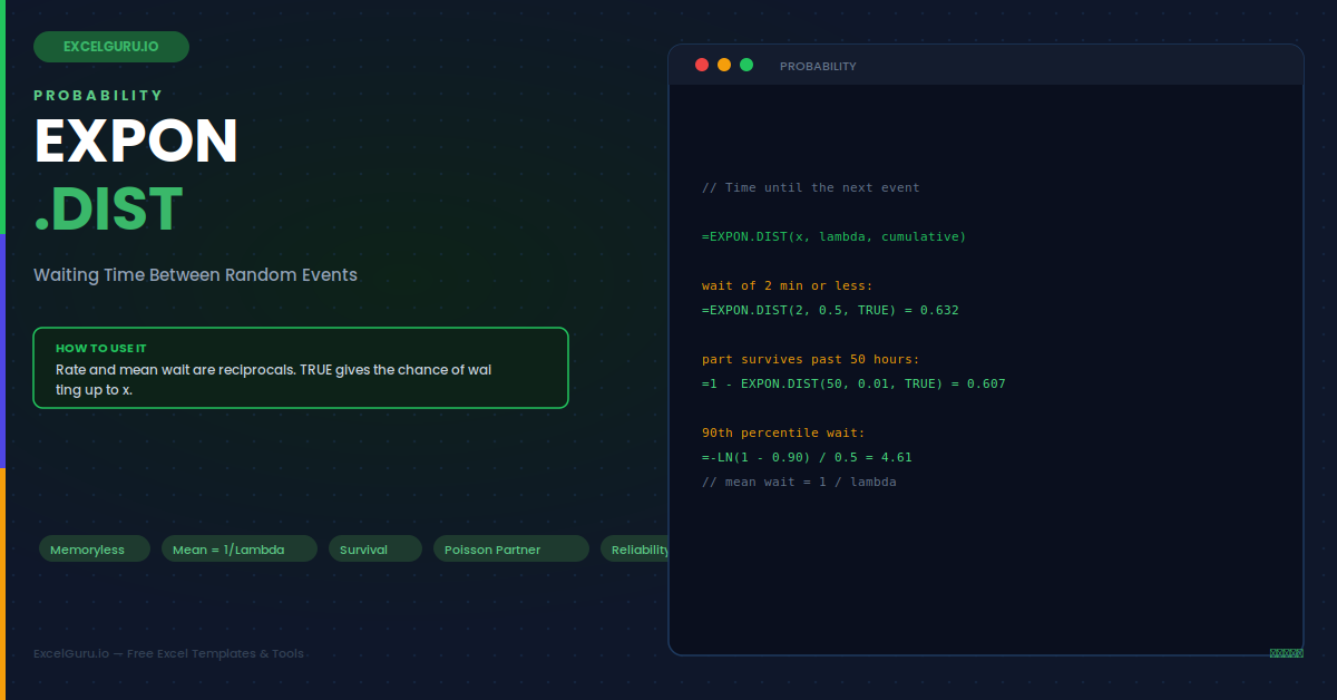
How long until the next customer walks in? How long before a machine part fails? How much time passes between website visits? These questions are not about counting events. They are about the gap between them. When events happen randomly at a steady average rate, the waiting time follows the exponential distribution. Excel handles it with EXPON.DIST. You give it a time value and a rate, and it returns the probability. It is the natural partner to the Poisson distribution.
This guide explains the exponential distribution in plain language. First, it shows how it links to the Poisson. Then it covers the rate input and the cumulative switch. Seven worked examples and a full troubleshooting section follow. By the end, you will model waiting times and reliability with a single function.
What the Exponential Distribution Models
The exponential distribution describes the time between random events. Those events occur at a steady average rate. The key insight is simple: short waits are common, long waits are rare. The probability drops off smoothly as time grows. The infographic below shows this decay curve.
Notice how the curve starts high and falls away. This means a short gap is the most likely outcome. However, very long gaps still happen occasionally. Consequently, the distribution captures the unpredictable nature of random arrivals. It never reaches zero, so an extremely long wait is always possible. That long tail is a defining feature.
The Link to the Poisson Distribution
The exponential and Poisson distributions are two sides of one coin. The Poisson counts events in a fixed interval. The exponential measures the time between those events. If calls arrive at three per hour, both describe the same process. One counts, the other times.
The Syntax and the Cumulative Switch
EXPON.DIST takes three arguments. The first is a time value. The second is the rate. The third is the cumulative switch, which again changes the meaning entirely.
Example 1: Probability of a Short Wait
Start with the most common question. What is the chance the wait is under a certain time? You set cumulative to TRUE. This gives the area under the curve up to that point.
Example 2: Probability of a Long Wait
Sometimes the long tail matters. What is the chance of waiting more than a set time? You use the complement rule. Because the total is 1, you subtract the cumulative value. This answers overflow and capacity questions directly.
Example 3: Reliability and Time to Failure
Engineering uses the exponential for failure times. Suppose a component fails at a rate of 0.01 per hour. You want the chance it survives 50 hours. That is the probability the failure time exceeds 50.
Example 4: The Memoryless Property
The exponential has a famous quirk: it is memoryless. The chance of waiting another minute does not depend on how long you have already waited. In other words, the process has no memory of the past. This surprises many people at first.
Example 5: Find a Time for a Given Probability
You can work backward to find a time. Suppose you want the time by which 90% of events occur. You rearrange the cumulative formula. This gives a percentile of the waiting time.
Example 6: Build a Survival Curve
A survival curve shows the chance of lasting past each time. You list a column of times. Then you compute one minus the cumulative for each. This traces how the survival chance decays.
Each survival value uses one minus EXPON.DIST with TRUE. The curve falls steadily over time. Notably, it reaches about 37% at the mean lifetime, a signature of the exponential. Plotting this column gives a clean survival chart. Reliability teams use it to picture how a population ages.
Example 7: Guard the Rate Input
The rate must be a positive number. A zero or negative rate has no meaning. A short guard flags a bad rate before calculating. This keeps a shared model tidy.
Troubleshooting EXPON.DIST
All three problems below are the most common. Each has a clear cause and a quick fix.
You get a #NUM! error
This error means an argument is invalid. The time value x cannot be negative, so a negative time fails at once. The rate lambda must be strictly greater than zero, because a zero or negative rate has no meaning. Check both arguments against these limits. A frequent slip is confusing the rate with the mean wait, which are reciprocals of each other. If you have the average wait, convert it first using lambda equals 1 divided by the mean. Once the time is non-negative and the rate is positive, the error clears.
The result is a strange height, not a probability
If EXPON.DIST returns an odd value that is not a probability, you likely set cumulative to FALSE. FALSE returns the height of the density curve at that point, not the area beneath it, and that height can even exceed 1. For an actual probability, the area up to a time, set cumulative to TRUE. This is the same trap that appears with other distribution functions. In nearly every practical case you want the cumulative version, so keep the switch on TRUE unless you specifically need the curve height.
The exponential does not fit my failure data
If the exponential does not match observed failures, the failure rate may not be constant. The exponential assumes a steady rate and the memoryless property, meaning age does not affect the chance of failing next. Real components often wear out, so older parts fail more readily, which breaks this assumption. In that case, the Weibull distribution is a better fit, because it allows the failure rate to rise or fall with age. Check whether your failure rate truly stays constant over time. When it does not, switch to a model that accounts for ageing.
Frequently Asked Questions
- What does the EXPON.DIST function calculate?+Essentially, EXPON.DIST calculates probabilities for the waiting time between random events that occur at a steady average rate. You provide a time value, the rate lambda, and a cumulative switch. When cumulative is TRUE, it returns the probability that the wait is at most that time, which is the most common use. When FALSE, it returns the height of the probability density curve at that point. For example, =EXPON.DIST(2, 0.5, TRUE) gives the chance the next event happens within 2 units of time at a rate of 0.5. It models arrival gaps and time-to-failure well.
- How are the rate and the mean related?+Specifically, the rate lambda and the mean waiting time are reciprocals of each other. The rate is the average number of events per unit of time, while the mean wait is the average time between events. So mean equals 1 divided by lambda, and lambda equals 1 divided by the mean. For example, a rate of 0.5 events per minute corresponds to an average wait of 2 minutes. This relationship is a frequent source of mistakes, because EXPON.DIST expects the rate, not the mean. If you know only the average wait, convert it to a rate first before using the function.
- What is the memoryless property?+Notably, the exponential distribution is memoryless, meaning the probability of waiting an additional amount of time does not depend on how long you have already waited. If a bus arrives on average every 10 minutes and you have already waited 5 minutes, your expected further wait is still 10 minutes, not 5. The process has no memory of the past. This property fits truly random arrivals, such as calls to a help desk, very well. However, it does not fit situations where age matters, like mechanical wear-out, where an older part is genuinely more likely to fail soon.
- When should I use Weibull instead of the exponential?+Use the exponential distribution when the failure or event rate is constant over time, which is its defining assumption. Switch to the Weibull distribution when the rate changes with age. The exponential is actually a special case of the Weibull, the one where the shape parameter equals 1 and the rate stays flat. Real components often show a rising failure rate as they wear out, or a falling rate during early break-in, and the Weibull captures both through its shape parameter. If your data shows that older items fail more or less often than new ones, the Weibull will fit far better than the exponential.