
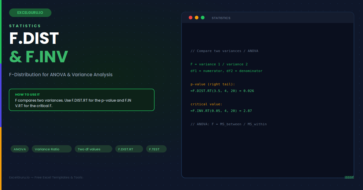
You have three machines, three suppliers, or three teams. Their average outputs look different. But are they really different, or is it just noise? A plain comparison of means will not settle it. You need to weigh the spread within each group against the spread between them. That is exactly what the F-distribution does. Excel exposes it through F.DIST and F.INV. These functions power the F-test and the whole method of ANOVA.
This guide explains the F-distribution without heavy maths. First, it shows what an F-ratio means. Then it covers each function variant. Seven practical examples cover variance comparison and ANOVA, followed by a full troubleshooting section. By the end, you will read an ANOVA table with confidence. You will also know how to verify every number in it yourself.
What the F-Distribution Measures
The F-distribution describes a ratio of two variances. In short, it compares how spread out two things are. Because it is a ratio of squared values, it can never be negative. It starts at zero and stretches to the right. This gives it a distinctive skewed shape. The infographic below shows the curve and its reject region.
When two variances are equal, the ratio sits near 1. A ratio far above 1 suggests a real difference. A ratio near 1 suggests none. Notably, the exact shape depends on two separate degrees of freedom. One comes from the top of the ratio, the other from the bottom. This two-part shape is what sets F apart from the t-curve.
The Two Degrees of Freedom
Unlike the t-distribution, the F-distribution needs two degrees of freedom. The first belongs to the numerator variance. The second belongs to the denominator variance. Both feed into every F function. Getting them in the right order matters.
The Function Variants Explained
Excel offers several F functions. Each returns a different part of the distribution. Choosing the right one depends on your question. The table below lays them out.
| Function | What it returns |
|---|---|
| F.DIST(x, df1, df2, TRUE) | Left-tail cumulative probability up to x |
| F.DIST.RT(x, df1, df2) | Right-tail probability beyond x (the p-value) |
| F.INV(prob, df1, df2) | Left-tailed F-value for a probability |
| F.INV.RT(prob, df1, df2) | Right-tailed critical F-value |
| F.TEST(array1, array2) | A two-tailed p-value comparing two variances directly |
Example 1: Get a p-value from an F-Ratio
Start with the core task. You have an F-ratio and want its p-value. The right-tail function gives it directly. A small p-value means the variances truly differ.
Example 2: Find a Critical F-Value
Sometimes you want the threshold instead. This is the critical F-value. You compare your F-ratio against it. F.INV.RT returns it for a chosen significance level.
Example 3: Compare Two Variances
A common use is testing whether two processes vary by the same amount. Consistency often matters as much as the average. A machine with steady output beats an erratic one. You take a sample from each. Then you form the ratio of their variances. The F-test tells you if the difference is real.
=VAR.S(range). Put the larger one on top.=larger_variance / smaller_variance.=F.DIST.RT(ratio, df1, df2).Example 4: The F-Test Behind One-Way ANOVA
ANOVA compares several group means at once. Testing each pair separately would inflate the error rate. ANOVA avoids that with a single test. It works by splitting the total variation into two parts. One part is variation between groups. The other is variation within groups. The F-ratio compares them. A large ratio points to a genuine group effect.
Example 5: Read the ANOVA Table Output
Excel can run ANOVA through the Analysis ToolPak. The output includes an F value and its p-value. Knowing the functions helps you read and verify that table. Here is how the pieces connect.
Here the F value is 5.2 and the p-value is 0.011. Because 0.011 is below 0.05, the group means differ significantly. You can confirm the p-value yourself with F.DIST.RT using the two df values from the table.
Example 6: Compare Critical Values Across df
The critical F-value shifts as degrees of freedom change. Larger samples give smaller critical values. This means bigger studies detect smaller differences. In other words, more data raises the power of the test. Seeing the pattern helps you plan a test. It shows why sample size is worth the effort.
With more denominator degrees of freedom, the critical value drops from 3.71 to 2.84. Therefore, a larger within-group sample makes the test more sensitive. This is a useful fact when designing experiments.
Example 7: A Safety Check Before an F-Test
A tidy model tests its inputs first. The F-test needs positive variances and valid degrees of freedom. Wrapping the logic in a check prevents confusing errors. This keeps a shared workbook clean.
Troubleshooting F.DIST and F.INV
All three problems below are the most common. Each has a clear cause and a quick fix.
You get a #NUM! error
This error points to an invalid argument. The x value in F.DIST must not be negative, because an F-ratio is always zero or positive. Check for a negative or wrongly calculated ratio. For F.INV and F.INV.RT, the probability must sit between 0 and 1. A value of 0, 1, or beyond fails. Both degrees of freedom must also be at least 1. Confirm df1 and df2 are whole positive numbers. Once every argument sits in its valid range, the error disappears.
The two degrees of freedom are swapped
Order matters with the F-distribution, and swapping df1 and df2 gives a wrong answer. The first degrees of freedom belong to the numerator variance, the one on top of the ratio. The second belong to the denominator variance. If your result looks off, check that each df matches its own variance. A common slip is pairing the numerator df with the denominator variance. Line up each variance with its own degrees of freedom, and the calculation returns the correct probability.
Results differ from an old FDIST formula
Older Excel used FDIST, which returned the right-tail probability directly. The modern F.DIST returns the left-tail cumulative value instead when the cumulative argument is TRUE. So FDIST(x, df1, df2) matches F.DIST.RT(x, df1, df2), not plain F.DIST. When updating an old workbook, map each legacy call to the correct new function. The difference is not an error but a change in which tail the function reports. Matching the tail explains almost every discrepancy between old and new sheets.
Frequently Asked Questions
- What is the F-distribution used for?+The F-distribution is used to compare variances, which makes it central to analysis of variance, or ANOVA. It describes the ratio of two variances, so it answers whether two or more groups spread out or differ by the same amount. In ANOVA, the F-ratio compares the variation between group means against the variation within the groups. A large ratio, and therefore a small p-value, means at least one group truly differs from the others. It also underlies simple two-sample variance comparisons and regression significance tests, wherever a ratio of variances needs a probability.
- Why does the F-distribution need two degrees of freedom?+Because the F-statistic is a ratio of two variances, each variance brings its own degrees of freedom. The first, df1, belongs to the numerator variance on top of the ratio. The second, df2, belongs to the denominator variance on the bottom. Together they define the exact shape of the curve. For a two-sample comparison, each equals its sample size minus one. In ANOVA, df1 comes from the number of groups minus one, and df2 comes from the total sample size minus the number of groups. Always keep each df matched to its own variance.
- Should I use F.DIST or F.DIST.RT for an F-test?+For a standard F-test you almost always want F.DIST.RT, which returns the right-tail probability, or p-value, beyond your F-ratio. Significance lives in the right tail because a large F-ratio signals a real difference in variances or means. Plain F.DIST with the cumulative argument TRUE returns the left-tail area instead, which is the probability up to your value rather than beyond it. To get the critical threshold for a chosen significance level, use F.INV.RT. Matching the right-tail functions to the right-tail logic of the test keeps your p-values and critical values consistent.
- How is the F-test related to ANOVA in Excel?+ANOVA is essentially a structured F-test across several groups. It splits the total variation into between-group and within-group parts, then forms an F-ratio by dividing the between-group mean square by the within-group mean square. Excel can run this automatically through the Analysis ToolPak, producing a table with an F value and its p-value. Behind that output sits the same F-distribution that F.DIST.RT uses. You can verify the reported p-value yourself with =F.DIST.RT(F, df_between, df_within), using the degrees of freedom shown in the ANOVA table.