ROUND, ROUNDUP, and ROUNDDOWN work in decimal places — they can give you 27.3 rounded to one decimal, but they cannot give you 27.3 rounded down to the nearest 5. That is what FLOOR and CEILING do. FLOOR always rounds down to the nearest multiple of a number you specify. CEILING always rounds up. The multiple can be 5, 10, 0.25, 0.05, or any other value — making these the right tools for rounding prices to coin denominations, quantities to box sizes, times to 15-minute slots, and scores to grade boundaries.
FLOOR and CEILING Syntax
| Argument | Required? | What it means |
|---|---|---|
| number | Required | The value to round. Usually a cell reference, but can be a hardcoded number or formula result. If the number is already an exact multiple of significance, it is returned unchanged. |
| significance | Required | The multiple to round to. FLOOR rounds down to the nearest value divisible by this number. CEILING rounds up. Common values: 5 (nearest 5), 0.05 (nearest 5 cents), 10 (nearest 10), 0.25 (nearest quarter-hour). |
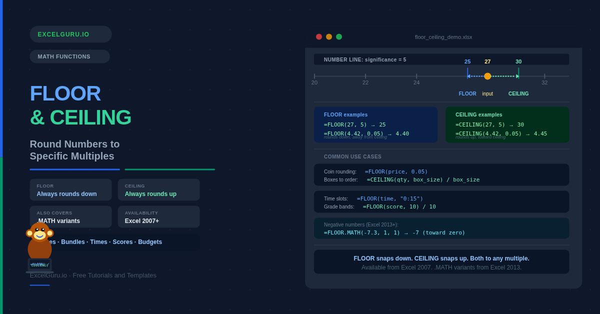
The visual below shows how FLOOR and CEILING work for the number 27, with significance 5. FLOOR finds the nearest multiple below; CEILING finds the nearest multiple above.
FLOOR, CEILING, and MROUND — Which One to Use?
| Feature | FLOOR | CEILING | MROUND |
|---|---|---|---|
| Direction | Always rounds down | Always rounds up | Rounds to nearest (up or down) |
| Multiple of 5 for 27 | 25 | 30 | 25 (nearer) or 30 |
| Multiple of 5 for 23 | 20 | 25 | 25 (nearer) |
| Guaranteed direction? | Yes — always down | Yes — always up | No — depends on value |
| Best use case | Floor quantities, lower price tiers | Bundle sizes, SLA windows, upper tiers | Time rounding, price rounding to nearest |
Example 1: Round Prices to Coin Denominations
The most common real-world use — rounding calculated prices to the nearest denomination you accept as cash. Use FLOOR to round down to the nearest 5 cents, or CEILING to round up to avoid dealing in small coins entirely.
Example 2: Packing and Bundle Quantities
When items are sold or shipped in fixed bundle sizes, you need to know how many complete bundles to dispatch (use FLOOR — round down to the last complete bundle) or how many to order to cover a requirement (use CEILING — round up to the next full bundle).
Example 3: Round Times to 15-Minute Slots
FLOOR and CEILING work with time values when significance is expressed as a fraction of a day, or as a time string like "0:15". This makes them ideal for rounding time entries to billing intervals or calendar slot boundaries.
Example 4: Round to Nearest 5, 10, or 100
FLOOR and CEILING round to any integer multiple, not just fractions. Use significance values of 5, 10, 50, 100, or 1000 to round scores, populations, budgets, or any large number to a clean reporting unit.
Example 5: Grade Boundaries and Score Tiers
FLOOR is ideal for assigning scores to grade bands — round down to the start of each 10-point tier and the result is the band label. Combine with CHOOSE or a lookup to convert the floored value into a letter grade or category.
Example 6: FLOOR.MATH and CEILING.MATH — Better Negative Number Handling
The original FLOOR and CEILING functions can behave unexpectedly with negative numbers — particularly if number and significance have mismatched signs. FLOOR.MATH and CEILING.MATH (Excel 2013+) add a mode argument that gives you explicit control over rounding direction for negative values.
Troubleshooting FLOOR and CEILING Errors
#DIV/0! error
The significance argument is 0. FLOOR and CEILING cannot round to a multiple of zero — it is mathematically undefined. Check the cell or formula providing the significance value and ensure it is non-zero.
#VALUE! error
One of the arguments is non-numeric. Verify that both number and significance cells contain numbers, not text. A cell displaying "5" but stored as text will cause this error.
#NUM! error (older Excel)
In Excel 2007 and Excel 2010, CEILING returns #NUM! if number is positive and significance is negative. Ensure both arguments share the same sign, or upgrade to CEILING.MATH which handles mixed signs without error.
Result is farther from zero than expected for negative numbers
FLOOR on a negative number rounds toward negative infinity by default — so FLOOR(-7.3, 1) returns -8, not -7. If you need rounding toward zero for negatives, use FLOOR.MATH with mode = 1.
=FLOOR(A2*100, 10)/100. For financial calculations with pennies, multiplying by 100 and working in integer cents eliminates floating-point surprises.
Frequently Asked Questions
-
What is the difference between FLOOR and CEILING in Excel?+FLOOR always rounds down to the nearest multiple of the significance value you specify. CEILING always rounds up. Both functions round to multiples rather than decimal places — significance 5 means "round to the nearest 5", not "5 decimal places". If a number is already an exact multiple, both functions return it unchanged.
-
What is the difference between FLOOR and ROUNDDOWN?+ROUNDDOWN rounds to a specified number of decimal places — ROUNDDOWN(27.83, 1) gives 27.8. FLOOR rounds to a specified multiple — FLOOR(27.83, 5) gives 25. Use ROUNDDOWN when you need a fixed number of decimal places. Use FLOOR when you need to snap to a specific multiple like 5, 10, 0.25, or 0.05.
-
What is the difference between CEILING and MROUND?+MROUND rounds to the nearest multiple — it can go either up or down depending on which multiple is closer. CEILING always rounds up to the next multiple, regardless of how close the number is to the one below. Use MROUND when you want standard rounding to the nearest multiple. Use CEILING when you must guarantee rounding up — for example, when calculating the number of boxes needed to fulfil an order.
-
How do I round a time to the nearest 15 minutes with FLOOR or CEILING?+Excel times are stored as fractions of a day — 15 minutes is 15/1440 or 1/96. You can pass the time string "0:15" directly as the significance argument: =FLOOR(A2, "0:15") or =CEILING(A2, "0:15"). Format the result cell as Time to display it correctly. For 30-minute rounding use "0:30", for hourly use "1:00".
-
When should I use FLOOR.MATH and CEILING.MATH instead of FLOOR and CEILING?+Use FLOOR.MATH or CEILING.MATH when working with negative numbers and you need explicit control over rounding direction, or when you want to omit the significance argument to round to the nearest integer (significance defaults to 1 in the .MATH variants). For positive numbers the results are identical to the original functions. FLOOR.MATH and CEILING.MATH require Excel 2013 or later.
-
How do I round prices to the nearest 5 cents with CEILING?+Use a significance of 0.05: =CEILING(A2, 0.05). This rounds the price up to the nearest multiple of $0.05. For example, $4.42 becomes $4.45 and $9.97 becomes $10.00. To round down to the nearest 5 cents instead (for customer-friendly pricing), use FLOOR(A2, 0.05) — $4.42 becomes $4.40.