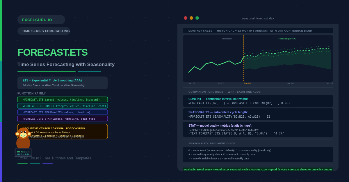
Most sales data follows a pattern: higher in December, slower in January, up again in spring. A simple average or trend line ignores that rhythm entirely. FORECAST.ETS accounts for it. It uses Exponential Triple Smoothing — an algorithm that separates trend from seasonal cycles and projects both forward. The result is a seasonally-aware forecast — it rises and falls with the cycle, not one that treats every future period as identical.
This guide covers the complete FORECAST.ETS function family: FORECAST.ETS for point forecasts, FORECAST.ETS.CONFINT for confidence intervals, FORECAST.ETS.SEASONALITY to detect cycle length automatically, and FORECAST.ETS.STAT to inspect the model’s internal parameters. Six practical examples cover building a seasonal forecast, adding uncertainty bands, detecting seasonality, validating the model, and handling gaps.
What Is Exponential Smoothing?
Exponential smoothing is a forecasting method that weights recent observations more heavily than older ones. The “exponential” name refers to how weights decrease as data gets older. Last month matters more than six months ago. Six months ago matters more than two years ago. Simple exponential smoothing handles level only. Double smoothing adds a trend component. Triple smoothing — also called Holt-Winters — additionally adds a seasonal component, and that is exactly what FORECAST.ETS implements.
Excel’s implementation uses the AAA variant: Additive errors, Additive trend, and Additive seasonality. This means the seasonal pattern is added on top of the trend line rather than multiplied by it. The additive model works best when seasonal peaks and troughs are roughly the same size regardless of the trend level. When seasonal swings grow proportionally with the trend, a multiplicative model is more appropriate. However, that requires tools outside Excel.
What Functions Are in the FORECAST.ETS Family?
| Function | What it returns | When to use it |
|---|---|---|
| FORECAST.ETS | A point forecast value for a future target date | Primary forecasting function. Use for any date or array of dates beyond the historical data. |
| FORECAST.ETS.CONFINT | The half-width of the confidence interval at a given target date | Add and subtract from FORECAST.ETS to get the upper and lower bounds of the forecast range. |
| FORECAST.ETS.SEASONALITY | The detected season length (e.g. 12 for monthly with annual cycles) | Let Excel detect the cycle length automatically, then use the result as the seasonality argument. |
| FORECAST.ETS.STAT | A specific statistic about the fitted model (alpha, beta, gamma, MAPE, etc.) | Inspect model quality and smoothing parameters after fitting. |
What Is the Syntax for FORECAST.ETS?
| Argument | Required? | What it does |
|---|---|---|
| target_date | Required | The date or number to forecast. Can be a single date or an array of future dates. Must be consistent with the timeline interval (e.g., monthly if the timeline is monthly). |
| values | Required | The historical values to fit the model to. A column of numbers — sales, units, revenue, any numeric time series. Cannot be empty. |
| timeline | Required | The dates or time steps corresponding to the values. Must be evenly spaced. Excel accepts small gaps and fills them using the data_completion argument. |
| seasonality | Optional | The length of one seasonal cycle. 1 = no seasonality. 0 = auto-detect (default). 12 = annual pattern in monthly data. 4 = annual pattern in quarterly data. Maximum value is 8,760. |
| data_completion | Optional | How to handle missing timeline points. 1 = interpolate missing values (default). 0 = treat missing as zero. |
| aggregation | Optional | How to aggregate duplicate timestamps. 1 = AVERAGE (default). Other options: 2=COUNT, 3=COUNTA, 4=MAX, 5=MEDIAN, 6=MIN, 7=SUM. |
Examples 1–4: Core Forecasting Patterns
The fundamental use is passing historical dates and values to FORECAST.ETS with a future target date. The function fits a seasonal model to the history and returns the predicted value for the requested period. Using an array of future dates in target_date produces a full forecast column automatically — no copy-paste required in Excel 365.
A point forecast alone is incomplete. Every prediction carries uncertainty, and that uncertainty grows with distance from the last observation. FORECAST.ETS.CONFINT returns the half-width of the confidence interval. Add it for the upper bound, subtract it for the lower bound. The confidence level argument controls how wide the interval is.
Before committing to a seasonality value, use FORECAST.ETS.SEASONALITY to let Excel report what it detects in the data. The function returns the length of one seasonal cycle as an integer. For monthly retail data this is typically 12. For quarterly revenue data it is typically 4. You can then pass this result directly as the seasonality argument in FORECAST.ETS to ensure consistency.
FORECAST.ETS.STAT exposes the model’s internal parameters and accuracy metrics. The statistic_type argument selects which value to return. Alpha controls how fast the model responds to level changes. Beta controls trend sensitivity. Gamma controls seasonal adjustment speed. MAPE — Mean Absolute Percentage Error — is the most useful accuracy metric for business reporting.
Examples 5 and 6: Applied Forecasting Scenarios
Forecast Charts and Missing Data Handling
A forecast is most useful when visualised alongside the historical data it was fitted to. The standard layout uses three forecast columns (point forecast, lower bound, upper bound) alongside the historical values in a line chart. Excel’s built-in Forecast Sheet (Data tab → Forecast Sheet) generates this layout automatically. Building it manually gives more control over the date range and confidence level.
Real datasets often have missing months, skipped periods, or irregular gaps. FORECAST.ETS handles minor gaps automatically when data_completion = 1 (the default). It interpolates the missing values internally before fitting the model. For intentionally excluded periods, set data_completion = 0 to treat missing points as zero. Note that this usually degrades forecast quality.
Common Issues and How to Fix Them
#VALUE! error from FORECAST.ETS
FORECAST.ETS returns #VALUE! when the timeline is uneven, when values and timeline have different lengths, or when target_date does not match the timeline type. Check that every row in the timeline column follows the same interval. Also confirm that text-formatted dates in the timeline are converted to genuine date values — =DATEVALUE(A2) converts a text date to a serial number Excel recognises.
The forecast ignores seasonality despite setting seasonality = 12
FORECAST.ETS needs at least two complete seasonal cycles to detect and model the pattern reliably. With 12 months of monthly data, the model has only one cycle and cannot establish a seasonal pattern. Consequently, the forecast falls back to trend-only behaviour. Provide at least two full cycles: 24 months for monthly seasonality, or eight quarters for quarterly seasonality.
Forecast values seem too low or too high overall
Check the MAPE from FORECAST.ETS.STAT(values, timeline, 8). A MAPE above 20% suggests the model is fitting poorly. This often happens because of a structural break — a sudden level change from a product launch, price change, or external event. In that case, trim the history to start after the break and refit the model on the more recent data.
Frequently Asked Questions
-
What is the difference between FORECAST.ETS and FORECAST.LINEAR?+FORECAST.LINEAR fits a straight trend line through the historical data and projects it forward. It is fast and simple, but it has no seasonal component — it cannot capture the recurring peaks and troughs that most business data exhibits. FORECAST.ETS fits an exponential smoothing model with separate level, trend, and seasonal components. It produces a curved, seasonally adjusted forecast. Use FORECAST.LINEAR for data with a clear trend but no seasonality. Use FORECAST.ETS whenever the data shows repeating seasonal patterns.
-
How much historical data does FORECAST.ETS need?+FORECAST.ETS requires at least two full seasonal cycles for reliable seasonal modelling. For monthly data with annual seasonality, that means at least 24 months of history. For quarterly data, at least eight quarters. With less than two cycles, the function can still return a result but it falls back to trend-only behaviour — the seasonal component is unreliable with too few cycles. More history generally improves accuracy, though very old data from a structurally different period can degrade the fit.
-
What does the MAPE statistic tell me and what is a good value?+MAPE — Mean Absolute Percentage Error — is the average percentage by which the model’s in-sample predictions differed from actual values. A MAPE of 0.05 means the model was off by 5% on average during the fitting period. For most business forecasting, a MAPE below 10% indicates a good fit. Between 10% and 20% is acceptable but worth investigating. Above 20% suggests the model may not be suitable for the data — check for structural breaks, insufficient history, or missing seasonality specification.
More Questions About FORECAST.ETS
-
Can FORECAST.ETS forecast weekly or daily data?+Yes. FORECAST.ETS works with any evenly spaced numeric timeline, including daily and weekly data. For daily data with a weekly cycle, set seasonality = 7. For weekly data with an annual cycle, set seasonality = 52. Auto-detection (seasonality = 0) also works for these frequencies when enough history is available. Be aware that daily data requires at least 14 days of history for weekly seasonality, and weekly data requires at least 104 weeks for annual seasonality detection.
-
What is the aggregation argument and when do I need it?+The aggregation argument handles duplicate timestamps in the timeline — for example, if the same date appears twice because two transactions were recorded on that day. The default is 1 (AVERAGE), which averages the values for duplicate timestamps before fitting. Other options are 2 (COUNT), 3 (COUNTA), 4 (MAX), 5 (MEDIAN), 6 (MIN), and 7 (SUM). For most business datasets where data is already aggregated to monthly or quarterly periods, duplicates do not appear and the default is fine. Set aggregation = 7 (SUM) if your data has daily transactions that need summing to a monthly timeline.
-
Is there a way to adjust the forecast for known future events?+FORECAST.ETS has no built-in mechanism for adding known future adjustments. The standard approach is to run the baseline forecast and then apply manual adjustments in a separate column. For example, if a promotional campaign is planned for March that typically boosts sales by 15%, multiply the March forecast by 1.15 in a separate adjusted-forecast column. This keeps the statistical baseline clean while allowing judgement-based overlays. Some analysts also reserve the most recent periods as a hold-out set to measure how accurately the model predicts known past data before trusting its future projections.