Excel's ribbon Sort button permanently reorders your data with no live connection and no automatic refresh. The Forecast Sheet feature on the Data tab is entirely different. It projects a time series forward using the same Exponential Triple Smoothing (ETS) algorithm used in enterprise forecasting platforms. The output is a new worksheet containing a chart, a forecast table, and statistical confidence bounds — created in one click from any two-column date-and-values dataset. This guide covers every dialog option, how to validate forecast quality by backtesting, and the FORECAST.ETS function family for embedding live forecasts directly in your models.
How ETS Forecasting Works
The ETS algorithm decomposes your historical data into three components. First, the baseline level of the series. Second, a trend component capturing whether values are rising or falling. Third, a seasonal component capturing repeating patterns at a fixed cycle length. Recent observations are weighted more heavily than older ones using smoothing parameters (alpha, beta, gamma). The confidence interval — shown as a shaded band in the chart — widens the further you project into the future because uncertainty compounds over time.
Data Requirements
Before running Forecast Sheet, five conditions must be met. The date column must contain true Excel date values, not text strings — left-aligned cells indicate text dates requiring conversion. Dates must be evenly spaced with no skipped intervals. You need at least 12 data points, though 24 or more is recommended for reliable seasonal detection. Data must be sorted chronologically, oldest first. The date column must contain plain dates, not datetime values with time components.
=DATEVALUE(A2) and paste-special as Values to replace the originals.The Forecast Sheet Dialog Options
After selecting any cell in your two-column data range and going to Data > Forecast > Forecast Sheet, the dialog opens with a live chart preview. The Options panel at the bottom controls six settings.
Example 1: Monthly Revenue — 12-Month Projection
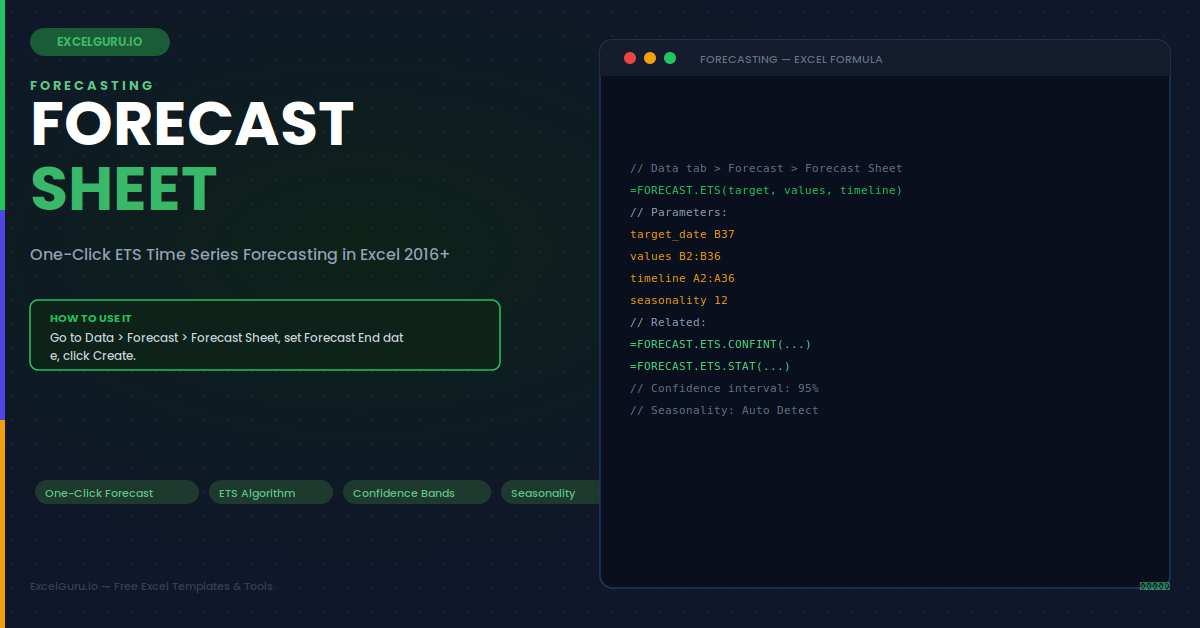
With 24 months of monthly revenue data, click inside the two-column table and go to Data > Forecast > Forecast Sheet. Set Forecast End to 12 months from the last data point. The output worksheet shows three columns for every future month: the Forecast value, the Lower 95% bound, and the Upper 95% bound. These three numbers directly feed an annual operating plan as the central, pessimistic, and optimistic revenue scenarios without any additional formula work.
Example 2: Daily Web Traffic — Manual Seasonality
Website session data shows a clear weekly pattern — lower on weekends, higher on weekdays. For daily data with a weekly cycle, set Seasonality manually to 7 in the Options panel. Auto Detect requires at least two complete cycles and may misidentify the length on sparse data. A 90-day projection at the correct weekly seasonality setting supports content planning schedules, server capacity decisions, and advertising spend optimisation by day of the week.
Example 3: Inventory Safety Stock from the Upper Bound
The upper confidence bound is not just an error margin — it is a demand risk estimate. The gap between the upper bound and the forecast value represents the additional stock needed to cover demand variability at the chosen confidence level. Run Forecast Sheet for each SKU separately with a 90-day horizon. For each future period, safety stock equals the upper bound minus the forecast value. This approach is statistically more precise than rule-of-thumb formulas and adapts automatically as the seasonal demand pattern evolves.
Example 4: Backtesting — Validate Forecast Quality
Before trusting any forecast for real decisions, validate the model by setting the Forecast Start date 6–12 months before the end of your historical data. The model trains on the earlier portion and forecasts the later portion — which you then compare against the actual known values. MAPE below 10% indicates an excellent model. MAPE between 10–20% is acceptable for most planning purposes. Above 20%, review the seasonality setting and check for data quality issues such as outliers or structural breaks in the history.
Example 5: FORECAST.ETS — Live Formula-Based Forecasting
Forecast Sheet creates a static snapshot that does not update when source data changes. For a live, auto-refreshing forecast value embedded in a dashboard or planning model, use the FORECAST.ETS worksheet function. It uses the identical ETS algorithm and recalculates every time the source data changes — particularly powerful when the source is an Excel Table that automatically expands as new monthly data is added. The related function family extends FORECAST.ETS with confidence bounds, model statistics, and seasonal cycle detection.
Example 6: Call Centre Staffing from Forecast Bands
Call centres use historical call volume to plan shift staffing. The forecast value drives baseline headcount. The upper confidence bound drives peak staffing to prevent queue buildup during high-demand shifts. The lower bound identifies the minimum viable staffing for cost control. This approach correctly captures seasonal volume patterns — higher volumes at month-end or during specific seasons — rather than applying a flat percentage uplift that ignores the actual shape of the historical pattern entirely.
Troubleshooting Forecast Sheet
Most Forecast Sheet problems have one of three root causes: text dates, insufficient history, or an incorrect seasonal cycle. Checking these three things in order resolves the majority of issues.
The Forecast Sheet button is greyed out
This almost always means the date column contains text strings formatted as dates rather than true Excel date values. Right-click a date cell and choose Format Cells — if the category shows "General" or "Text", the dates need converting. Use =DATEVALUE(A2) and paste-special as Values to replace the column. Also verify you clicked inside the data range before opening the dialog, not on an adjacent blank cell.
The forecast is a flat line with no trend or seasonality
A flat forecast means ETS detected insufficient variation to model trend or seasonality — typically because fewer than two complete seasonal cycles are present in the history. Fix it by setting Seasonality manually in the Options panel to the expected cycle length: 12 for monthly data with an annual pattern, 7 for daily data with a weekly pattern, 4 for quarterly data. Also check whether outliers or one-off events are confusing the pattern detection algorithm.
The confidence interval is extremely wide
Very wide bands indicate high historical volatility relative to the forecast horizon. Three things widen the bands: a long forecast horizon, high historical variance, and a high confidence level setting. To narrow the bands, reduce the Confidence Interval percentage from 95% to 80%, or shorten the forecast horizon. If genuine outliers from one-off events are present in the history, smoothing or removing them before forecasting produces narrower and more representative confidence bands.
Frequently Asked Questions
- How many data points does Forecast Sheet require?+Excel requires at least 12 data points to run a forecast. For reliable seasonality detection, however, you need at least two complete seasonal cycles — 24 months minimum for monthly data with an annual pattern. More history generally produces more reliable results, though recent data is weighted more heavily by the ETS algorithm. If you have fewer than two cycles, set Seasonality manually rather than relying on Auto Detect, which requires at least two complete repetitions to identify the cycle length.
- What is the difference between Forecast Sheet and FORECAST.ETS?+Forecast Sheet is a wizard that creates a static snapshot on a new worksheet, complete with a chart and confidence bounds table. FORECAST.ETS is a worksheet formula that returns a single forecast value and recalculates automatically when source data changes. Both use the identical ETS algorithm and produce the same numerical output for the same inputs. Use Forecast Sheet for exploring, presenting, or backtesting a forecast. Use FORECAST.ETS for live dashboards and planning models where the forecast must stay current as new data arrives.
- Can Forecast Sheet handle missing values in the historical data?+Yes. The Options panel includes a "Fill Missing Using" setting. Interpolation (the default) fills gaps by linearly interpolating between surrounding known values — the correct approach for most time series. Zeros fills missing periods with zero, appropriate only when absence genuinely means no activity rather than a recording gap. For long consecutive gaps (three or more missing periods), filling values manually with reasonable estimates before running the forecast produces more reliable results than automatic interpolation alone.
- Does Forecast Sheet work for fiscal year data?+Yes. Forecast Sheet does not require calendar year alignment. It reads the date column directly and detects patterns based on the interval between consecutive dates, regardless of where the year boundary falls. For fiscal year data, use fiscal period end dates in the date column and the corresponding values in the values column. The ETS algorithm detects seasonal patterns from the data itself. For live fiscal year forecasts in models, FORECAST.ETS combined with the DATESYTD DAX pattern in Power Pivot provides the most flexible approach.