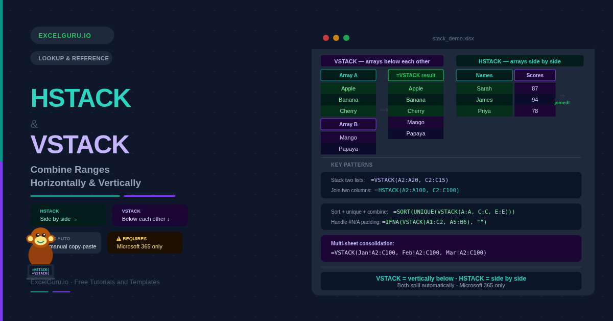
Merging data from separate ranges has always required copying, pasting, and then re-sorting. Every time the source data changes, you repeat the process. The VSTACK function eliminates this entirely — it stacks multiple ranges vertically into a single dynamic output that updates automatically. Similarly, the HSTACK function places ranges side by side in a single horizontal array. Both outputs spill automatically and respond instantly to changes in the source data.
Together, VSTACK and HSTACK unlock a new class of formula-driven reporting — consolidating monthly tables, combining filtered results, and assembling dynamic dashboards without any manual copy-paste steps. Furthermore, they combine naturally with SORT, UNIQUE, and FILTER to create powerful data pipelines in a single formula.
What Is the Syntax for VSTACK and HSTACK?
Both functions take a simple list of arrays or ranges, separated by commas.
| Argument | Required? | What it does |
|---|---|---|
| array1 | Required | The first range or array to include. Can be a cell range, a named range, an array constant, or the result of any formula that returns an array. |
| array2… | Optional | Additional ranges to stack. Up to 254 arrays are supported. Each is appended below (VSTACK) or to the right (HSTACK) of the previous array. |
How Do VSTACK and HSTACK Differ?
The choice between them is simple — it comes down to which direction the data should grow.
| Feature | VSTACK | HSTACK |
|---|---|---|
| Direction | Vertical — arrays stack below each other | Horizontal — arrays sit side by side |
| Result width | Widest array's column count | Sum of all arrays' column counts |
| Result height | Sum of all arrays' row counts | Tallest array's row count |
| #N/A padding when | Arrays have different column counts | Arrays have different row counts |
| Best for | Consolidating monthly tables, combining filtered lists | Assembling side-by-side columns, building report headers |
Example 1: Combine Two Lists Vertically with VSTACK
VSTACK appends one list below another and spills the result automatically. The output is fully live — if either source list grows, the combined result grows too. No formula editing is needed. This makes VSTACK ideal for consolidating data that arrives in separate batches.
Example 2: Place Ranges Side by Side with HSTACK
HSTACK appends columns to the right of the previous array. This is useful for assembling separate columns of data that belong in the same report — for instance, joining a list of names from one table with corresponding scores from another, or building a dynamic header row from separate arrays.
Example 3: Handle Different-Size Arrays and #N/A Errors
When stacked arrays have different dimensions, the smaller one is padded with #N/A errors to fill the gap. VSTACK pads missing columns. HSTACK pads missing rows. Both situations are easy to handle — wrap the entire VSTACK or HSTACK formula in IFERROR or IFNA to replace the errors with a blank or a default value.
Example 4: VSTACK + SORT + UNIQUE — The Data Pipeline
VSTACK is most powerful when combined with other dynamic array functions. A common pattern is to stack multiple lists, remove duplicates with UNIQUE, and sort the result — all in a single formula. Additionally, pairing VSTACK with FILTER lets you consolidate only the rows that meet a condition across multiple source ranges.
Example 5: Build a Dynamic Report Table with HSTACK
HSTACK lets you assemble report tables from separate formula results. Instead of placing calculated columns across a sheet manually, you can chain them horizontally and produce a self-contained, sorted, filterable report in one formula block. Moreover, inserting a blank-column separator keeps the layout visually clean.
=SEQUENCE(COUNTA(A2:A100)) generates exactly as many row numbers as there are entries — so the rank column always has the right length. No hardcoding needed. Adding new data automatically extends the numbering.
Example 6: Consolidate Data from Multiple Sheets
Before VSTACK existed, pulling data from multiple sheets into one required Power Query or complex INDIRECT formulas. VSTACK handles this directly — you can reference ranges on different sheets as separate arguments. As a result, a single formula consolidates all sheet data into one live output.
Using VSTACK Across Sheets
Each argument can reference a different sheet using the standard SheetName!Range syntax. Consequently, new data added to any source sheet appears automatically in the combined output. Furthermore, combining this with UNIQUE removes any rows that appear on more than one sheet.
=FILTER(VSTACK(...), VSTACK(...)<>"").
How to Fix Common HSTACK and VSTACK Issues
#N/A errors in the output
These appear when stacked arrays have different dimensions. VSTACK adds #N/A to missing columns. HSTACK adds #N/A to missing rows. The fix is straightforward — wrap the formula in =IFNA(VSTACK(...), "") to replace the errors with blank cells. Alternatively, use 0 if the column contains numbers that feed into calculations.
#SPILL! error
A #SPILL! error means the formula's output range is blocked by existing data. Either delete the cells in the spill range or move the formula to a location with enough clear space. Additionally, check whether another formula or a merged cell is occupying the output area.
Output includes blank rows from oversized source ranges
If you use a larger range than the data fills — for instance, A2:A100 when only 20 rows are populated — VSTACK includes the blank rows in the output. Consequently, wrap in FILTER to remove them: =FILTER(VSTACK(A2:A100, C2:C100), VSTACK(A2:A100, C2:C100)<>""). Alternatively, use Excel Tables as the source — Table references automatically exclude empty rows.
Frequently Asked Questions
-
What is the difference between VSTACK and HSTACK?+VSTACK stacks arrays vertically — each additional array appears below the previous one. HSTACK, by contrast, stacks arrays horizontally — each additional array sits to the right of the previous one. Use VSTACK when you want to combine rows from different sources into one tall list. Use HSTACK when you want to combine columns from different sources into one wide table. Both functions spill automatically and update when the source data changes.
-
Why am I getting #N/A errors in my VSTACK result?+The #N/A errors appear because the stacked arrays have different numbers of columns. VSTACK pads the narrower arrays with #N/A to match the widest array. To fix this, wrap the formula in IFNA: =IFNA(VSTACK(array1, array2), ""). This replaces every #N/A with a blank. Use 0 instead of "" if the column should remain numeric for downstream calculations.
-
How do I combine VSTACK with SORT and UNIQUE?+Nest the functions in order — VSTACK produces the combined array, UNIQUE removes duplicates, and SORT orders the result: =SORT(UNIQUE(VSTACK(A2:A20, C2:C15, E2:E30))). Because Excel evaluates from the inside out, VSTACK runs first, then UNIQUE, then SORT. The entire output spills automatically from the cell where you enter the formula.
More Questions About HSTACK and VSTACK
-
Can VSTACK combine ranges from different sheets?+Yes. Each argument can reference a different worksheet using the standard SheetName!Range syntax: =VSTACK(January!A2:C100, February!A2:C100, March!A2:C100). The formula combines all three sheets into one output automatically. New rows added to any source sheet appear in the combined output without any formula changes. Pair with FILTER to exclude blank rows from oversized ranges.
-
How do I add a header row to a VSTACK or HSTACK result?+Include an array constant as the first argument of VSTACK: =VSTACK({"Name","Score"}, HSTACK(A2:A100, B2:B100)). The curly-brace array creates the header row. VSTACK then appends the data below it. Each value in the array constant becomes a column header matching the corresponding column in the stacked result. This produces a complete, labelled table from a single formula.
-
Which Excel versions support HSTACK and VSTACK?+Both functions are available only in Microsoft 365 (the subscription version). They work in Excel for the web and Google Sheets as well. Notably, they are not available in Excel 2021, Excel 2019, Excel 2016, or any earlier standalone versions — those display a #NAME? error. For cross-version files, use Power Query or INDIRECT-based approaches to consolidate data across ranges.