Nested IF formulas are one of the most common sources of confusion in Excel. Each additional condition buries itself deeper inside the previous one, making the formula longer, harder to read, and easy to break. The IFS function replaces the entire nesting structure with a clean linear list of conditions — you simply write each test and its result in order, left to right. This guide covers the syntax, shows you a direct comparison with nested IF, and walks through six practical examples covering grading, commissions, pricing tiers, and more.
IFS Function Syntax
IFS takes pairs of arguments — a logical test followed by the value to return if that test is TRUE. It evaluates each pair from left to right and returns the value for the first TRUE condition it finds.
| Argument | Required? | What it means |
|---|---|---|
| logical_test1 | Required | The first condition to evaluate — any expression that returns TRUE or FALSE. |
| value_if_true1 | Required | The value returned when logical_test1 is TRUE. Can be text, a number, a formula, or a cell reference. |
| logical_test2, value_if_true2... | Optional | Additional condition and result pairs. Up to 127 pairs allowed. IFS stops at the first TRUE condition and ignores all remaining pairs. |
#N/A. To provide a fallback, add TRUE as the final logical_test with your default value: =IFS(A1>90,"A", A1>80,"B", TRUE,"C"). Since TRUE is always true, this last pair always catches anything not matched above.
IFS vs Nested IF — Side by Side
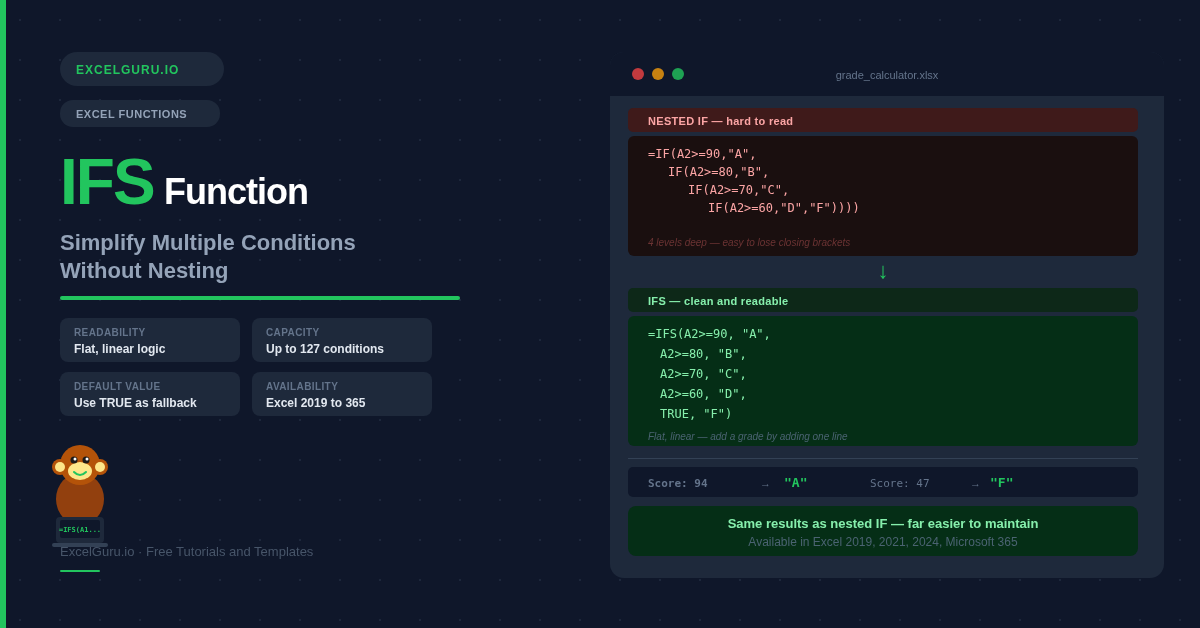
The most immediate benefit of IFS is readability. Here is the same logic written both ways — assigning letter grades from a score:
=IF(A2>=90,"A",
  IF(A2>=80,"B",
    IF(A2>=70,"C",
      IF(A2>=60,"D",
        "F"))))

4 levels of nesting.
Easy to lose closing brackets.
Hard to add a new grade band.
=IFS(A2>=90,"A",
     A2>=80,"B",
     A2>=70,"C",
     A2>=60,"D",
     TRUE,"F")

No nesting.
One bracket at the end.
Add a band by adding one line.
Both formulas produce identical results. The IFS version is visually easier to audit, easier to debug, and easier to hand off to a colleague who did not write it.
Example 1: Letter Grades from a Score
The classic use of IFS — assign a letter grade based on a numeric score. Each condition checks whether the score falls in a band, from highest to lowest. Order matters: IFS returns the first TRUE result, so always check the largest threshold first.
Example 2: Sales Commission Tiers
Tiered commission structures are a perfect fit for IFS — each revenue band maps to a commission rate, and the formula reads like a rate card. No helper columns, no lookup tables needed.
Example 3: Text Category Lookup
IFS works equally well when conditions match exact text values rather than numeric ranges. Use it to categorise products, map status codes to labels, or translate abbreviations into full names — all without a VLOOKUP or a lookup table.
Example 4: Shipping Method by Order Value
Business rules that assign categories based on numeric thresholds are exactly what IFS was designed for. Here, shipping method is determined by the order total — a common e-commerce and logistics scenario.
Example 5: Performance Rating with AND Conditions
Each logical_test in IFS can itself be a compound expression. Wrap AND or combine multiple comparisons to create conditions that require more than one criterion to be true — for example, assigning a performance rating based on both target attainment and customer score.
Example 6: IFS Inside Other Formulas
IFS is not limited to standing alone in a cell. You can nest it inside other functions — use it as the value inside an IF, wrap it with TEXT for formatting, or embed it inside CONCAT to build dynamic labels. It returns a value just like any other formula.
Troubleshooting IFS Errors
#N/A error — no condition is TRUE
IFS returns #N/A when none of your conditions evaluate to TRUE for a given row. The fix is simple: add TRUE as the final logical_test with a default value. Since TRUE is always true, it acts as a catch-all: =IFS(A1>90,"A", A1>80,"B", TRUE,"Other").
#VALUE! error — a condition does not return TRUE or FALSE
Every logical_test must evaluate to TRUE or FALSE. If a condition references a text cell with a numeric comparison, or contains a formula that returns an error, IFS returns #VALUE!. Test each condition individually in a blank cell — for example, type =(A2>=90) — to confirm it returns TRUE or FALSE as expected.
Wrong result — condition order is incorrect
IFS returns the first TRUE result and stops. If you check a lower threshold before a higher one, a high-scoring value will match the lower condition first. Always arrange numeric thresholds from most restrictive (highest) to least restrictive (lowest). Test with boundary values — a score of exactly 90 should confirm the right grade is returned.
IFS not available — using Excel 2016 or earlier
IFS was introduced in Excel 2019. If your version does not support it, the equivalent nested IF formula produces identical results. For many conditions, the CHOOSE or SWITCH functions may also be suitable alternatives depending on the structure of your logic.
Frequently Asked Questions
-
What does the IFS function do in Excel?+IFS evaluates a series of conditions from left to right and returns the value paired with the first condition that is TRUE. It replaces nested IF statements with a flat, readable list of test-result pairs. You can include up to 127 condition-value pairs in a single IFS formula.
-
How is IFS different from a nested IF?+Nested IF buries each additional condition inside the previous one, creating a deeply indented structure that is hard to read and easy to break with mismatched brackets. IFS lists all conditions at the same level, left to right, making the formula much easier to write, read, and extend. The logic is identical — IFS is simply a cleaner syntax for the same operation.
-
How do I add a default value to IFS?+Add TRUE as the final logical_test, followed by your default value: =IFS(A1>=90,"A", A1>=80,"B", TRUE,"Other"). Since TRUE is always true, this final pair catches every case not matched by the earlier conditions. Without it, IFS returns #N/A when no condition is met.
-
Which Excel versions support IFS?+IFS is available in Excel 2019, Excel 2021, Excel 2024, and Microsoft 365. It is not available in Excel 2016 or earlier. If you share workbooks with colleagues on older Excel versions, use nested IF instead to ensure compatibility.
-
Why is the order of conditions important in IFS?+IFS returns the value for the first TRUE condition and immediately stops evaluating. For numeric range checks, this means you must arrange conditions from most restrictive to least restrictive. For example, check A1>=90 before A1>=80 — otherwise a score of 95 would match the A1>=80 condition first and return the wrong grade.
-
When should I use IFS instead of SWITCH or VLOOKUP?+Use IFS when your conditions involve ranges or comparisons — greater than, less than, between. Use SWITCH when you are matching one value against a fixed list of exact values (like code 100 = "OK", 200 = "Warning"). Use VLOOKUP or XLOOKUP when you have a large mapping table that is likely to change, since a lookup table is easier to maintain than a formula when you have many possible values.