
Excel has two tools for answering "what value should this cell be?". Goal Seek finds the input that produces one specific target output, but it handles only one variable and one constraint. Solver, the free Add-in on the Data tab, extends this to any number of decision variables and any number of constraints simultaneously. It finds the optimal values for the decision variables — maximising profit, minimising cost, or hitting a specific target — subject to every constraint you define. It handles linear programming, non-linear optimisation, and integer programming: the same problem classes used in operations research, supply chain planning, and financial portfolio optimisation. This guide covers all three solving methods, six complete worked examples, and every common troubleshooting scenario.
Enabling Solver
Solver is a free Excel Add-in that ships with every version of Excel but is not enabled by default. Enable it once and it remains available until you uninstall Office or reset Excel options. After enabling, the Solver button appears on the Data tab in the Analyse group at the far right of the ribbon.
The Three Required Inputs
Every Solver model requires exactly three inputs. Understanding each one clearly before building the model prevents the most common setup errors and avoids confusing Solver with the entirely different Goal Seek tool.
- Objective Cell — the single formula cell you want to maximise, minimise, or set to a specific value. It must reference the decision variable cells directly or through formulas. This is the thing you are trying to optimise.
- Variable Cells — the cells Solver is allowed to change. These are the decision variables — the quantities, allocations, or selections you want to find the optimal values for. Solver changes these cells iteratively until the objective is optimised.
- Constraints — limits on the variable cells and on other cells in the model. For example: quantities must be non-negative, total budget must not exceed £200k, staffing must meet minimum coverage requirements per shift. Each constraint is a formula relationship (<=, =, >=) between a cell reference and a value.
Example 1: Product Mix — Maximise Profit with Resource Constraints
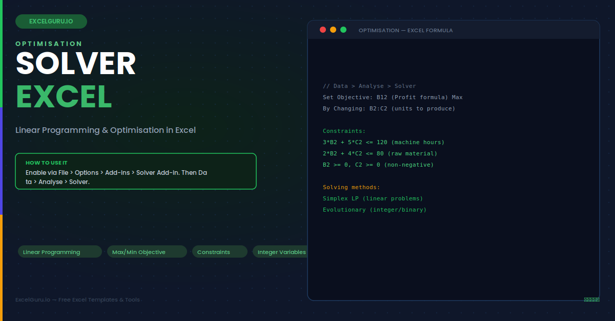
A factory produces Widget A and Widget B. Each requires different amounts of machine time and raw material, both of which are limited. The question is: how many of each product should be produced to maximise total profit? This is the classic linear programming product mix problem — all relationships are linear, so Simplex LP finds the exact global optimum in milliseconds. The objective, constraints, and variable ranges are all set up in Excel cells before opening the Solver dialog.
Example 2: Portfolio Optimisation — Maximise Return Within Risk Limit
An investor has £100,000 to allocate across five asset classes. Each has a historical return rate and a risk score. The goal is to maximise expected return while keeping portfolio risk below a specified threshold. Additionally, no single asset class may exceed 40% of the total portfolio. When return and risk are both calculated as weighted sums of the allocation amounts, all relationships are linear — making this a Simplex LP problem with a guaranteed global optimum.
Example 3: Workforce Scheduling — Minimum Cost with Coverage Requirements
A call centre must staff specific minimum agent counts for each hour of the day. Staff work 8-hour shifts starting at different hours. The goal is to find the minimum number of staff per shift that meets all hourly coverage minimums at the lowest total cost. Because the number of staff per shift must be whole numbers, this is an integer programming problem — it specifically requires the Evolutionary solving method rather than Simplex LP. Integer constraints are added using "int" in the constraint operator dropdown.
Example 4: Transportation Problem — Minimum Cost Distribution
A company has three warehouses and four distribution centres. Each warehouse has a supply limit. Each centre has a demand requirement. Specific shipping costs apply per unit for each warehouse-to-centre route. The transportation problem finds shipment quantities meeting all supply and demand requirements at minimum total shipping cost. This is one of the foundational linear programming problem types and is solved exactly by Simplex LP, typically in under one second regardless of the model size.
Example 5: Capital Budgeting — Select Projects with Binary Variables
A company has 8 investment projects to evaluate. Each has a required capital outlay and an expected net present value (NPV). The total capital budget is limited. The company wants to select the combination of projects that maximises total NPV without exceeding the budget. Each project is either fully selected (1) or not selected (0) — no partial investment is permitted. Binary integer variables are added to Solver using the "bin" option in the constraint dialog, and the Evolutionary method is required.
Example 6: Blending — Cheapest Mix Meeting Nutrient Specifications
A fertiliser manufacturer blends four raw materials to produce a compound product that must meet minimum nutrient content specifications. Each raw material has a different cost per unit and different nutrient content percentages. The blending problem finds the proportion of each raw material that meets all minimum nutrient specifications at the lowest possible cost. This is a standard linear programming application in food manufacturing, chemical blending, feed production, and pharmaceutical compounding industries.
Troubleshooting Solver
All three issues below are the most common problems users encounter when running Solver for the first time. Each has a clear diagnostic step that confirms the cause quickly.
Solver finds no feasible solution
A "no feasible solution" message means no combination of decision variable values simultaneously satisfies all constraints. This occurs because the constraints are contradictory — requiring both X > 100 and X < 50 simultaneously, for example — or the budget or resource limits are too tight for the demand constraints to be met. Review each constraint individually. Temporarily relax or remove constraints one at a time to identify which combination is causing the infeasibility. Once the conflicting constraints are identified, adjust them to reflect realistic resource limits.
Solver finds a solution but the result does not seem optimal
For non-linear problems solved with GRG Nonlinear, the solution may be a local optimum rather than the global optimum. GRG can get trapped at a local peak or valley depending on the starting values in the decision variable cells. Fix this by enabling "Use Multistart" in Solver Options, which runs GRG from multiple random starting points and compares results — typically finding the global optimum for well-behaved non-linear models. Alternatively, switch to the Evolutionary method for non-smooth or multimodal objective functions.
Solver runs but the values do not change and the objective stays the same
This typically means the objective cell formula does not reference the decision variable cells — even indirectly through other formulas. Solver can only improve the objective by changing the variable cells. If those changes do not affect the objective cell's formula, the objective stays constant regardless of what Solver does. Trace the formula precedents of the objective cell (Formulas > Trace Precedents) to confirm it connects to the variable cells. Also verify the decision variable cells are not locked by cell protection, which prevents Solver from writing new values to them.
Frequently Asked Questions
- How do I enable Solver in Excel?+Go to File > Options > Add-ins. At the bottom of the dialog, ensure "Manage: Excel Add-ins" is selected and click Go. Check the Solver Add-in checkbox and click OK. Solver will then appear on the Data tab in the Analyse group. It is available in all versions of Excel for both Windows and Mac and is included at no extra cost with every Excel installation. You only need to enable it once — it remains enabled across sessions until you explicitly uncheck it.
- What is the difference between the three Solver solving methods?+Simplex LP solves linear programming problems where all relationships between variables, objective, and constraints are strictly linear — no multiplication of variables by each other, no exponentials or logarithms. It is the fastest method and guarantees finding the global optimum. GRG Nonlinear handles smooth non-linear problems but may find only a local optimum. Evolutionary uses a genetic algorithm for non-smooth, discontinuous, or integer and binary variable problems. Use Simplex LP whenever possible, and verify your model is truly linear before choosing this method.
- How do I add integer or binary constraints in Solver?+In the Solver Parameters dialog, click Add to create a constraint. Select the decision variable cell or range on the left. In the middle dropdown, choose "int" for whole numbers or "bin" for binary (0 or 1 only). Click OK. Integer and binary constraints require the Evolutionary solving method — Solver will warn you and offer to switch automatically when these constraint types are detected. Binary constraints are appropriate for yes/no decision problems: selecting projects, assigning staff to shifts, choosing suppliers.
- Can Solver handle problems with hundreds of variables and constraints?+Yes, within limits. The standard Excel Solver handles up to 200 decision variables and up to 100 constraints for Simplex LP, and up to 200 variables for GRG Nonlinear and Evolutionary. For larger models, Frontline Systems (the Solver developer) offers commercial "Premium Solver" products that handle thousands of variables and hundreds of thousands of constraints. For supply chain, logistics, and large financial optimisation problems beyond the standard Solver limits, Python libraries such as PuLP, SciPy.optimize, and Gurobi provide significantly larger capacity and faster solve times.