TREND gives you predictions. LINEST gives you the whole story. Where TREND returns a single column of fitted values, LINEST returns a table of statistics: slopes, intercept, R², standard errors, F-statistic, degrees of freedom, and the regression sum of squares. These are the numbers that tell you not just what the model predicts, but how reliable those predictions are. LINEST is Excel’s gateway to full linear regression analysis without leaving the spreadsheet.
This guide covers every row and column of the LINEST output array, the syntax for simple and multiple regression, and eight practical examples. Specifically, you will learn how to extract individual statistics, build a prediction with confidence, run a multiple regression with several predictors, and assess whether the model is statistically meaningful. No statistical software is required for any of these tasks.
What Does LINEST Do?
LINEST fits a straight line through your data using ordinary least squares. For multiple predictors, it fits a hyperplane. The line minimises the sum of squared vertical distances between the actual data points and the fitted line. LINEST then returns a two-dimensional array of statistics: regression coefficients in row 1, standard errors in row 2, R² and standard error of the estimate in row 3, F-statistic and degrees of freedom in row 4, and the regression and residual sums of squares in row 5.
The key distinction from TREND is purpose. Specifically, each function serves a different analytical goal. TREND is for prediction — feed it new x-values and it returns predicted y-values. LINEST is for analysis — it returns the model parameters and their statistical properties. You can also build predictions from LINEST output, but the primary use is understanding the fit, which predictors matter, and whether results are statistically significant.
What Is the LINEST Syntax?
| Argument | Required? | What it does |
|---|---|---|
| known_y | Required | The dependent variable values (the outcome you are predicting). A single column of numbers. |
| known_x | Optional | The independent variable values (predictors). A single column for simple regression. Multiple columns for multiple regression. If omitted, Excel uses {1, 2, 3, ...}. |
| const | Optional | TRUE (default) = fit the intercept normally. FALSE = force the intercept through zero (regression without a constant). |
| stats | Optional | TRUE = return the full 5-row statistics table. FALSE (default) = return only the coefficients in row 1. Always use TRUE for regression analysis. |
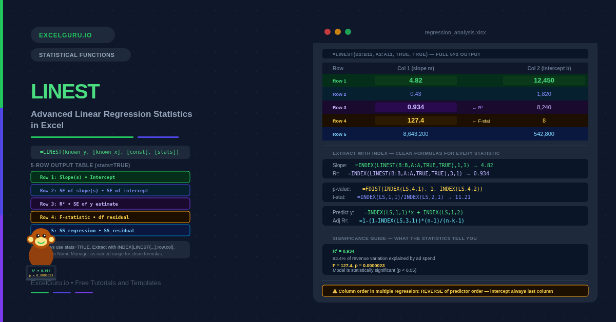
What Does the LINEST Output Table Contain?
The full LINEST output is a 5-row by (k+1)-column array, where k is the number of predictor variables. For simple regression with one predictor, the output is 5 rows × 2 columns. For multiple regression with three predictors, it is 5 rows × 4 columns. The columns are ordered from the last predictor to the first, with the intercept always in the rightmost column.
Examples 1–4: Core LINEST Operations
The starting point for any LINEST analysis is simple regression: one predictor, one outcome. The output gives you the slope (how much y changes per unit of x), the intercept (the y value when x equals zero), and R² (what fraction of the variation in y the model explains). These three numbers summarise the entire linear relationship.
Once you have the slope and intercept from LINEST, prediction is a matter of applying y = mx + b. Storing the coefficients in named cells avoids recalculating LINEST every time. The result matches TREND exactly — both use the same underlying least-squares fit. However, LINEST additionally gives you the standard error of the estimate, which allows you to build a prediction interval around the forecast.
R² tells you how much variance the model explains, and the F-statistic tests whether that is statistically meaningful. Specifically, it tests whether the explanatory power could have arisen by chance. A p-value below 0.05 means the model is significant at the 5% level. Excel’s FDIST function converts the F-statistic and degrees of freedom from LINEST into a p-value directly.
The F-statistic tests overall model significance. Standard errors from row 2, however, test whether each individual coefficient is significant. Dividing a coefficient by its standard error gives the t-statistic. Generally, an absolute t-statistic above 2 indicates significance. The TDIST function converts the t-statistic and degrees of freedom to a precise p-value.
Examples 5–8: Applied Regression Analysis
Multiple Regression, Polynomial Curves, and Residuals
Multiple regression extends the single-predictor model to include several independent variables simultaneously. For example, revenue might depend on both ad spend and headcount. LINEST handles this by passing a multi-column range as known_x. The output grows by one column per additional predictor. Importantly, coefficients appear in reverse predictor order — the rightmost column is always the intercept.
LINEST fits linear models — but the predictors do not have to be raw x-values. By passing x² (x squared) as a second predictor alongside x, you fit a quadratic (parabolic) curve. This is polynomial regression implemented through LINEST’s multiple regression framework. The curve fits data that bends rather than following a straight line, making it useful for diminishing returns, U-shaped cost curves, and accelerating growth.
Residuals are the differences between the actual y-values and the values the model predicted. Specifically, examining residuals is the primary diagnostic tool in regression. Well-behaved residuals are randomly scattered around zero with no pattern. Systematic curves in residuals indicate that a linear model is not appropriate. Furthermore, a single large residual can signal an outlier or a data entry error.
A self-updating regression report is one of the most practical uses of LINEST. Store the LINEST call in a named range, then extract each statistic with INDEX. This builds a self-updating dashboard. Every time the data changes, all statistics refresh simultaneously without any manual intervention.
Common Issues and How to Fix Them
LINEST only returns one number instead of the full table
Two things cause this. First, stats may be FALSE or omitted — set stats = TRUE to get all five rows. Second, in Excel 2019 and earlier, LINEST must be entered as an array formula: select the full output range (5 rows × (k+1) columns), type the formula, then press Ctrl+Shift+Enter. Without this, only the top-left value is returned. In Excel 365, LINEST spills automatically and no special entry is needed.
The column order in LINEST output is confusing
LINEST returns coefficients in reverse order of the predictor columns. For simple regression, column 1 is the slope and column 2 is the intercept — straightforward. For multiple regression with three predictors passed as columns A, B, C, the LINEST output columns are the coefficient for C, then B, then A, then the intercept. Always use INDEX(LINEST(...), 1, col) to extract specific coefficients rather than relying on visual column position in the spilled array.
R² is high but the model still gives poor predictions
High R² does not guarantee useful predictions. Several issues can inflate R² without producing a reliable model. Consequently, R² alone is not a reliable quality indicator. Overfitting is the most common issue. Adding more predictors always increases R², even if those predictors are irrelevant. Instead, use Adjusted R² (Example 8), which penalises extra predictors. Also check the residuals — if they show a systematic pattern, the linear model is misspecified and predictions will be unreliable regardless of R².
Frequently Asked Questions
-
What is the difference between LINEST and TREND?+TREND returns predicted y-values for a set of x-values. It is a prediction tool. LINEST returns the regression coefficients and statistical diagnostics — slope, intercept, R², standard errors, F-statistic, and sums of squares. It is an analysis tool. Both use identical least-squares fitting, so a prediction from LINEST coefficients always matches TREND exactly. Use TREND when you only need predictions. Use LINEST when you need to understand and validate the model.
-
How do I use LINEST in Excel 2019 and earlier?+In Excel 2019 and earlier, LINEST is an array function. To get the full 5-row output, select a 5×2 range (or 5×(k+1) for multiple regression), type the LINEST formula, and confirm with Ctrl+Shift+Enter instead of Enter. Curly braces appear in the formula bar to confirm array entry. If you only need one statistic — for example, just R² — you can wrap LINEST in INDEX and enter it in a single cell normally: =INDEX(LINEST(B2:B11,A2:A11,TRUE,TRUE),3,1) does not require Ctrl+Shift+Enter.
-
What is R² in LINEST and what is a good value?+R² (the coefficient of determination) measures what proportion of the variation in y is explained by the model. It ranges from 0 to 1. An R² of 0.90 means 90% of the variation in y is explained. What counts as a good value depends entirely on the field. In physics, R² should be near 1.0. In economics or social science, 0.50 to 0.70 may be perfectly acceptable. A high R² does not mean the model is well-specified — always check residuals and use Adjusted R² when comparing models with different numbers of predictors.
More Questions About LINEST
-
How do I extract the slope and intercept from LINEST?+Use INDEX to extract specific cells from the LINEST array. For simple regression, the slope is in row 1, column 1: =INDEX(LINEST(B2:B11,A2:A11,TRUE,TRUE),1,1). The intercept is in row 1, column 2: =INDEX(LINEST(B2:B11,A2:A11,TRUE,TRUE),1,2). For multiple regression, the column order reverses relative to the predictor order — the last predictor’s coefficient is in column 1, the first predictor’s coefficient is in column 2, and the intercept is always in the last column. Store the LINEST output in a named range for cleaner formulas.
-
What is the const argument in LINEST?+The const argument controls whether the model includes a free intercept. When const = TRUE (the default), LINEST fits both the slope and intercept freely to best match the data. When const = FALSE, the intercept is forced to zero — the regression line is constrained to pass through the origin. Use FALSE only for theoretically justified models where a zero x-value must correspond to a zero y-value. For most business and scientific applications, leave const as TRUE. Forcing a zero intercept when it is not theoretically justified biases the slope estimate.
-
Can LINEST handle non-linear relationships?+LINEST itself only fits linear models. However, you can fit non-linear curves by transforming the predictors before passing them to LINEST. For a quadratic curve, pass both x and x² as predictors (polynomial regression, shown in Example 6). For an exponential curve, take the natural log of y and fit a linear model to ln(y) vs x. For a power curve, take logs of both x and y. These transformations make the relationship linear in the transformed variables, which LINEST can then fit. The resulting model is still estimated by ordinary least squares, just applied to the transformed data.