Average and median tell you the centre of a dataset. They say nothing about where any individual value sits relative to everyone else. Rank-based metrics fill that gap. They answer a different and often more useful question: not "what is typical?" but "where does this value rank?" A sales figure is not just a number — it is top 10%, bottom quartile, or 73rd percentile. PERCENTILE and QUARTILE functions give you those answers directly in Excel.
This guide covers the complete PERCENTILE and QUARTILE function family — PERCENTILE.INC, PERCENTILE.EXC, QUARTILE.INC, QUARTILE.EXC, and PERCENTRANK.INC — and the RANK function for whole-number ranking. Eight practical examples show how to use them for performance banding, outlier detection, compensation analysis, grading curves, and executive dashboards. By the end, you will know exactly which function to reach for in any ranking scenario.
What Are Percentiles and Quartiles?
A percentile tells you the value below which a given percentage of observations fall. Specifically, the 90th percentile is the value below which 90% of the data sits. Quartiles are percentiles at fixed intervals. Specifically, Q1 is the 25th percentile, Q2 is the 50th percentile (the median), and Q3 is the 75th. Together, Q1 and Q3 define the interquartile range (IQR) — the spread of the middle 50% of the data.
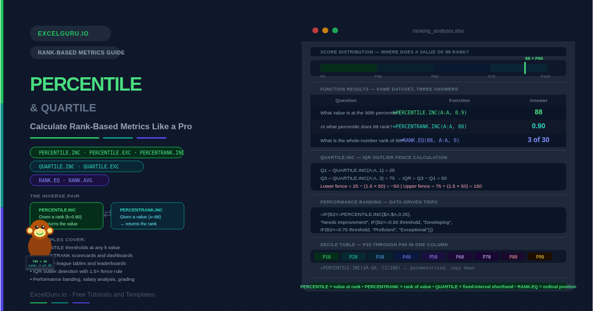
PERCENTRANK is the inverse operation. Essentially, it flips the question around. Instead of asking what value sits at the 90th percentile, it answers the reverse: at what percentile does this value sit? Both operations are essential for ranking work. PERCENTILE returns a value given a rank. PERCENTRANK returns a rank given a value.
What Functions Are in the PERCENTILE and QUARTILE Family?
| Function | What it returns | Key constraint | Replaces |
|---|---|---|---|
| PERCENTILE.INC | Value at a given percentile (0 to 1 inclusive) | k can be 0 or 1 (min/max) | Legacy PERCENTILE |
| PERCENTILE.EXC | Value at a given percentile (exclusive of 0 and 1) | k must be strictly between 0 and 1 | No legacy equivalent |
| QUARTILE.INC | Quartile value (quart 0–4 inclusive) | quart 0 = min, 4 = max | Legacy QUARTILE |
| QUARTILE.EXC | Quartile value (quart 1–3 exclusive) | quart 0 or 4 returns #NUM! | No legacy equivalent |
| PERCENTRANK.INC | Percentile rank of a value (0 to 1 inclusive) | Returns 0 for min, 1 for max | Legacy PERCENTRANK |
| PERCENTRANK.EXC | Percentile rank of a value (exclusive) | Never returns exactly 0 or 1 | No legacy equivalent |
| RANK.EQ | Whole-number rank of a value in a list | Ties receive the same rank | Legacy RANK |
What Is the Syntax for Each Function?
| Argument | Function | What it does |
|---|---|---|
| array / ref | All | The range of numeric values to rank against. Text and empty cells are ignored. |
| k | PERCENTILE.INC / EXC | The percentile as a decimal: 0.25 = 25th percentile, 0.9 = 90th percentile. INC accepts 0 and 1. EXC requires strictly between 0 and 1. |
| quart | QUARTILE.INC / EXC | Integer 0–4 for INC (0=min, 1=Q1, 2=median, 3=Q3, 4=max). Integer 1–3 for EXC — 0 and 4 return #NUM!. |
| x | PERCENTRANK.INC / EXC | The specific value whose percentile rank you want to find. Need not be in the array. |
| significance | PERCENTRANK.INC / EXC | Optional. Number of decimal places in the result. Default is 3 (e.g. 0.857). |
| order | RANK.EQ | 0 = rank largest as 1 (descending, default). 1 = rank smallest as 1 (ascending). |
Examples 1–4: Core Ranking Operations
PERCENTILE.INC answers one question: what value marks the Nth percentile in my dataset? It is the most frequently used ranking function. It is ideal for setting performance thresholds, pay band boundaries, and benchmark targets. The k argument is a decimal between 0 and 1 — so the 90th percentile is k = 0.90.
PERCENTRANK.INC is the inverse of PERCENTILE.INC. It answers "at what percentile does this specific value rank?" The result is a decimal between 0 and 1. Multiply by 100 to get a whole-number percentile. It is specifically useful for individual scorecards, league table positions, and peer comparison reports.
PERCENTRANK returns a fractional percentile. RANK.EQ returns a whole-number position: 1st, 2nd, 3rd. This is the right function when your audience expects ordinal ranks — sports league tables, sales leaderboards, and student rankings all communicate better with positions than with percentile decimals. Ties receive the same rank; the next rank is skipped.
The interquartile range (IQR) is Q3 minus Q1. The standard outlier rule flags values below Q1 − 1.5×IQR or above Q3 + 1.5×IQR. Store Q1, Q3, and IQR in named cells. This avoids recalculating those values repeatedly and keeps the outlier flag formula readable.
Examples 5–8: Applied Scenarios
Performance Banding, Compensation, and Dashboards
Performance reviews often use three or four tiers: Needs Improvement, Developing, Proficient, and Exceptional. Defining those bands using PERCENTILE.INC makes them data-driven and self-updating. As new scores are added to the dataset, the thresholds adjust automatically — no manual recalculation required.
Salary analysis uses quartile bands to assess pay equity. Specifically, comparing an individual's salary to the Q1 and Q3 of their job grade tells you whether they are at risk of leaving (below Q1) or paid above market (above Q3). Additionally, the midpoint — Q2 — is a common target for competitive market positioning.
Norm-referenced grading assigns letter grades based on where students rank relative to their cohort — not against a fixed score scale. The top 10% receive an A. The next 25% receive a B. The middle 30% receive a C, and so on. PERCENTILE.INC calculates the score thresholds automatically for any cohort size.
Executive dashboards often need a complete distributional summary alongside individual performance cards. A decile table — showing the value at every 10th percentile from P10 to P90 — gives a full picture of the distribution in nine rows. Pairing it with PERCENTRANK and RANK.EQ for the featured metric also creates a self-contained ranking summary that updates as data changes.
Common Issues and How to Fix Them
PERCENTILE.EXC returns #NUM!
PERCENTILE.EXC requires k to be strictly between 0 and 1 — it returns #NUM! for k = 0 or k = 1 exactly. It also returns #NUM! when the dataset has too few values for the requested percentile. On small datasets with k very close to 0 or 1 (such as 0.01 or 0.99), switch to PERCENTILE.INC instead. It handles those boundary positions without error.
PERCENTRANK gives an unexpected decimal
PERCENTRANK.INC returns a value between 0 and 1, not a whole-number percentage. Multiply by 100 and wrap in ROUND to get a clean integer: =ROUND(PERCENTRANK.INC(A:A, B2)*100, 0). The result also depends on every value in the reference array — adding or removing data changes all PERCENTRANK results. For a stable rank that does not shift with new data, use RANK.EQ instead.
RANK.EQ produces gaps after tied values
When two values tie for rank 3, RANK.EQ assigns both rank 3 and skips rank 4 — the next value is rank 5. This is statistically correct but can surprise audiences expecting consecutive numbers. If you need a dense ranking with no gaps — where ties share a rank but the next rank is not skipped — use COUNTIF instead: =COUNTIF($B$2:$B$100,">"&B2)+1 for a descending dense rank.
Frequently Asked Questions
-
What is the difference between PERCENTILE.INC and PERCENTILE.EXC?+Both functions find the value at a given percentile position, but they use different interpolation methods. PERCENTILE.INC treats k = 0 as the dataset minimum and k = 1 as the maximum, including those boundary values in the calculation. PERCENTILE.EXC excludes those boundaries — k must be strictly between 0 and 1. As a result, PERCENTILE.EXC returns a slightly lower value at the same k for most datasets. PERCENTILE.INC matches R, Python, and Google Sheets by default. PERCENTILE.EXC matches TI-84 calculators and many academic textbooks. Use INC for most business work.
-
What is the difference between PERCENTILE and PERCENTRANK?+They are inverse operations. PERCENTILE takes a percentile position (k = 0.90) and returns the corresponding value. PERCENTRANK takes a specific value (x = 88) and returns its percentile position (0.90). Use PERCENTILE when you want to know "what value is at the 90th percentile?" Use PERCENTRANK when you want to know "at what percentile does this specific value sit?"
-
What is the difference between RANK.EQ and RANK.AVG?+Both functions rank a value in a list. When there are no ties, they return identical results. The difference appears only on tied values. RANK.EQ assigns the same rank to all tied values (the lowest rank in the group), then skips the next ranks. RANK.AVG assigns the average of the ranks those tied values would have occupied. For example, two values tied for ranks 3 and 4 both receive rank 3.5 from RANK.AVG and rank 3 from RANK.EQ. Use RANK.EQ for leaderboards and ordinal rankings. Use RANK.AVG for statistical analysis where average tied ranks are needed.
More Ranking Questions
-
How do PERCENTILE and QUARTILE relate to each other?+Quartiles are percentiles at fixed positions. QUARTILE.INC(data, 1) always returns the same value as PERCENTILE.INC(data, 0.25). Similarly, QUARTILE.INC(data, 3) equals PERCENTILE.INC(data, 0.75). QUARTILE is a convenient shorthand for the specific percentile cuts at 25%, 50%, and 75%. For any other percentile position — the 10th, 33rd, 90th, or any non-quartile value — use PERCENTILE.INC or PERCENTILE.EXC directly.
-
Can PERCENTRANK return a value outside 0 to 1?+No. PERCENTRANK.INC always returns a value between 0 and 1 inclusive. It returns 0 for the minimum value in the array and 1 for the maximum. PERCENTRANK.EXC never returns exactly 0 or 1 — it returns a value strictly between those bounds. If you supply an x value that is outside the range of the array (below the minimum or above the maximum), PERCENTRANK returns #N/A because the value is outside the known data range.
-
How do I create a dense rank with no gaps after ties?+RANK.EQ skips ranks after ties — two values at rank 3 make the next value rank 5. To produce a dense rank where ties share a position and the next rank immediately follows, use COUNTIF: for a descending dense rank, =COUNTIF($B$2:$B$100,">"&B2)+1. For an ascending dense rank, =COUNTIF($B$2:$B$100,"<"&B2)+1. This approach never skips a rank number regardless of how many ties exist.