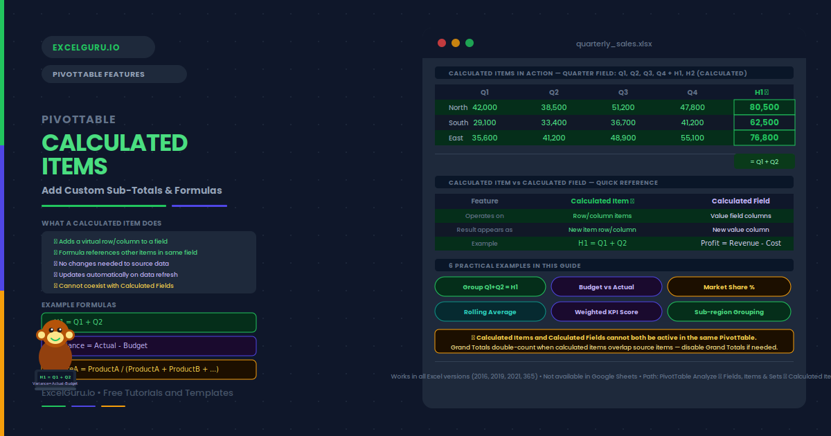
Your PivotTable shows Q1, Q2, Q3, and Q4. You want a row for H1 (Q1+Q2) and another for H2 (Q3+Q4) — without adding columns to the source data. Calculated Items make this possible. Each one inserts a virtual row or column. Its value comes from a formula referencing other items in the same field. The result appears in the PivotTable as if it were real data, but it lives entirely inside the PivotTable itself.
This guide explains what calculated items are and how they differ from calculated fields. It also covers creation, editing, and deletion. You will also learn when to use them, what their key limitations are, and six practical examples. Examples include grouping quarters into halves, computing market share, and creating a budget-versus-actual variance row.
What Are PivotTable Calculated Items?
A Calculated Item is a virtual item added to a PivotTable field. Its value is computed by a formula that references other items in the same field. For example, in a Region field with North, South, East, and West, you could add a calculated item called "Total Regions" defined as = North + South + East + West. That item then appears as a row or column alongside the real items.
Calculated items are different from calculated fields. A calculated field adds a new value column. Its formula combines existing value fields — for example, Profit = Revenue − Cost. A calculated item adds a new row or column entry. Its formula combines existing items within a row or column field. In short, calculated fields work on value columns. Calculated items work on category rows.
| Feature | Calculated Field | Calculated Item |
|---|---|---|
| Operates on | Value fields (columns) | Items in a row/column field |
| Result appears as | New value column | New row or column item |
| Formula references | Other value field names | Other item names in the same field |
| Example use | Profit = Revenue − Cost | H1 = Q1 + Q2 |
| Conflicts with | Calculated Items | Calculated Fields |
How Do You Create a Calculated Item?
Creating a Calculated Item takes just a few steps. First, click any cell in the field where you want the new item to appear — for example, click a cell in the Region row field to add an item to the Region field. Then navigate to the Calculated Item dialog.
= and can reference item names from the Items list on the right side of the dialog. Double-click an item name to insert it.Examples 1–6: Calculated Items in Practice
The Quarter field contains Q1, Q2, Q3, and Q4 as column labels. You want two additional columns — H1 and H2 — showing the first and second half totals. Adding calculated items to the Quarter field creates these groupings without touching the source data.
The Scenario field contains two items: Budget and Actual. Adding a calculated item called Variance shows the difference between them. Additionally, a Variance % item shows the relative difference as a fraction. Both update automatically when the underlying data changes.
The Product field contains Product A, Product B, and Product C. You want a row showing each product’s share of the total. A calculated item divides one item’s value by the sum of all items. This creates a percentage row directly in the PivotTable.
The Month field contains Jan through Dec as column items. A calculated item can average two adjacent months to produce a rolling two-period average. This is useful for smoothing noisy monthly data in a compact PivotTable view.
Examples 5–6: Advanced Calculated Item Patterns
The KPI field contains three items: Sales, Satisfaction, and Delivery. Each contributes a different weight to an overall performance score. A calculated item named Composite applies the weights in a single formula. This gives management a blended metric without modifying the source data.
The Region field contains eight sub-regions: NE, NW, SE, SW, MW-North, MW-South, Coast-N, and Coast-S. Management wants to see four summary regions: North, South, Midwest, and Coast. Instead of restructuring the source data, calculated items create these groupings on the fly.
Common Issues and How to Fix Them
The Calculated Item option is greyed out
This happens for two reasons. First, the active cell may not be inside a row or column field label — click a region label or quarter label rather than a value cell. Second, the PivotTable already contains a Calculated Field. Excel disables one when the other is present, since both conflict. Remove the Calculated Field first. Then add your Calculated Item.
The calculated item shows double-counted Grand Totals
This is the most common Calculated Item problem. When a calculated item sums existing items, the Grand Total row also adds those same items — plus the calculated item — resulting in double counting. The fix is to hide the Grand Total row via PivotTable Design → Grand Totals. Alternatively, design the calculated item so it does not replicate the Grand Total scope. Specifically, use them for sub-groupings only — not sums that overlap with the Grand Total.
Item names with spaces or special characters cause formula errors
Item names with spaces, hyphens, or special characters need single quotes inside the formula. For example, = 'MW-North' + 'MW-South' is correct, but = MW-North + MW-South returns an error because Excel interprets the hyphen as subtraction. Double-clicking an item in the Items panel inserts it with quotes automatically.
Frequently Asked Questions
-
What is a PivotTable Calculated Item?+A Calculated Item is a virtual entry added to a PivotTable row or column field. Its value comes from a formula that references other items in the same field. For example, you can add an H1 item to a Quarter field using the formula = Q1 + Q2. The item appears in the PivotTable alongside the real items, updates automatically when the source data changes, and requires no changes to the underlying dataset. Calculated Items differ from Calculated Fields, which add new value columns rather than new row or column entries.
-
What is the difference between a Calculated Item and a Calculated Field?+A Calculated Field adds a new column to the Values area by combining existing value fields. For example, Profit = Revenue minus Cost. A Calculated Item adds a new row or column to a row or column field by combining existing items in that field. For example, H1 = Q1 + Q2. They serve different purposes and cannot coexist in the same PivotTable. Use Calculated Fields when you need a new measure. Use Calculated Items when you need a new grouping or derived category.
-
Why does my PivotTable Grand Total look wrong after adding a Calculated Item?+Calculated Items cause double-counting in Grand Totals because the Grand Total includes both the original items and the calculated item, which itself references those same originals. For example, if Q1=100 and Q2=150 and you add H1=Q1+Q2, the Grand Total counts Q1, Q2, and H1 separately, summing to 100+150+250=500 instead of 250. The cleanest fix is to turn off Grand Totals for that axis, or to carefully design the Calculated Item so it represents a distinct non-overlapping group.
-
Can I use a Calculated Item with grouped date fields?+No. Calculated Items are not available when a date field is grouped using Excel's built-in date grouping (right-click → Group → Months, Quarters, Years). The Calculated Item option will be greyed out. In this case, add the custom groupings to the source data before building the PivotTable, or use a helper column in the data with the desired groupings already applied. Alternatively, use Power Query to add a custom period column before loading the data.