POISSON.DIST: Poisson Distribution for Rare Event Predictions

Home » pub » Tutorials » POISSON.DIST: Poisson Distribution for Rare Event Predictions

Master the POISSON.DIST function in Excel to calculate the probability of rare events occurring within a specific time, distance, or area. This tutorial explains the POISSON.DIST syntax, mean event rate, exact versus cumulative probabilities, interval-based rate adjustments, practical examples, and common errors. Learn how to calculate probabilities for calls per hour, production defects, accidents, website errors, and other count-based events, and understand when the Poisson distribution is more appropriate than the binomial distribution. Ideal for students, analysts, statisticians, researchers, quality-control professionals, and Excel users working with probability and forecasting.

A call centre averages three calls an hour. A stretch of highway sees two crashes a month. A website logs five errors a day. These are rare, countable events spread over time or space, arriving at some average rate. When you need the odds of a specific count, the Poisson distribution is the tool. Excel delivers it through POISSON.DIST. You give it a count and an average rate, and it returns the probability. With one cumulative switch, it also gives the chance of that count or fewer.

This guide explains the Poisson distribution without heavy maths. First, it shows when the model fits. Then it covers the single rate input and the cumulative switch. Seven worked examples and a full troubleshooting section follow. By the end, you will forecast rare-event counts with a single, simple function.

When to Use the Poisson Distribution

The Poisson distribution suits rare events over a continuous span. That span might be time, distance, or area. You need to know only one thing: the average rate. Unlike the binomial, there is no fixed number of trials. The infographic below shows a typical Poisson shape.

Think of arrivals at a help desk. You do not have a set number of trials, just an average flow. Similarly, defects along a production line follow this pattern. They appear at some steady rate per metre. Consequently, the Poisson models both cases with ease. It also covers accidents per month, typos per page, and arrivals per minute. Any rare, countable event with a steady rate fits the pattern.

Poisson vs Binomial

These two distributions are close cousins. Both count successes or events. However, they differ in one key way. The binomial needs a fixed number of trials. The Poisson only needs an average rate over an interval.

Which model fits your data: BINOMIAL: You have n fixed trials, each success or failure. Example: 20 parts tested, each pass or fail. POISSON: You have events over an interval, no fixed n. Example: calls per hour, defects per metre. Rule of thumb: if you can count trials, use binomial. If you only have an average rate, use Poisson.

The Syntax and the Cumulative Switch

POISSON.DIST takes just three arguments. Only one of them describes the process: the mean rate. The third is the familiar cumulative switch. As with the binomial, that switch changes everything.

Syntax: =POISSON.DIST(x, mean, cumulative) x -> the number of events you ask about. mean -> the average rate over the interval (lambda). cumulative -> TRUE = P(X <= x), a running total. FALSE = P(X = x), an exact count. Example: =POISSON.DIST(3, 3, FALSE) -> exactly 3 events. =POISSON.DIST(3, 3, TRUE) -> 3 events or fewer.

The mean is the whole model. The Poisson distribution is defined by its rate alone. For it, the mean and the variance are equal. So if events average three per hour, the variance is also three.

Example 1: The Exact Probability

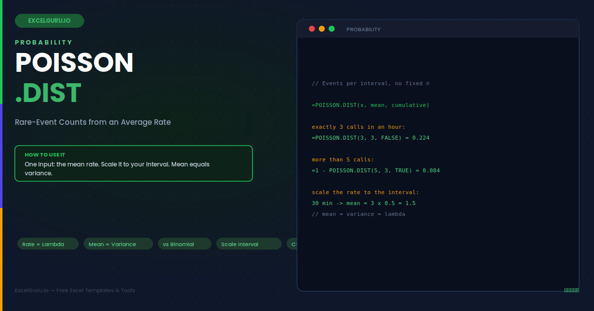
Start with a precise count. What is the chance of exactly three calls in an hour? You set cumulative to FALSE. This gives the probability of that count alone.

Exactly 3 calls in an hour: A call centre averages 3 calls per hour. =POISSON.DIST(3, 3, FALSE) Result: about 0.2240, or 22.40%. Reading it: there is roughly a 22% chance of getting exactly 3 calls in any given hour.

Example 2: The Cumulative Probability

Often a threshold matters more. What is the chance of three calls or fewer? You switch cumulative to TRUE. This sums the probabilities from zero through three.

3 calls or fewer: Same rate: 3 calls per hour on average. =POISSON.DIST(3, 3, TRUE) Result: about 0.6472, or 64.72%. Meaning: about a 65% chance of 3 or fewer calls. The cumulative version adds P(0)+P(1)+P(2)+P(3) for you in a single formula.

Example 3: The Probability of More Than X

Capacity planning often asks about overload. What is the chance of more than five calls? You use the complement rule. Because the total probability is 1, you subtract the cumulative value.

More than 5 calls in an hour: Average rate is 3 calls per hour. "More than 5" means "not 5 or fewer", so: =1 - POISSON.DIST(5, 3, TRUE) Result: about 0.0839, or 8.39%. Use case: if more than 5 calls overwhelms your staff, this says it happens about 8% of hours. That informs staffing decisions directly.

Example 4: Scale the Rate to a Different Interval

The rate must match the interval you ask about. If the average is per hour but you want a half-hour, you scale it. You simply adjust the mean to the new span. This is a common and important step. Skipping it is a frequent source of wrong answers.

Match the rate to the interval: Base rate: 3 calls per hour. For a 30-minute window, halve the mean: new mean = 3 * 0.5 = 1.5 =POISSON.DIST(2, 1.5, FALSE) -> chance of 2 in 30 min. For a 2-hour window, double the mean: new mean = 3 * 2 = 6 =POISSON.DIST(5, 6, TRUE) -> 5 or fewer in 2 hours. Always scale the mean to the interval you are asking about.

Example 5: A Real Quality-Control Use

Manufacturing uses Poisson for defect rates. Suppose a fabric averages two flaws per metre. You want the chance of a clean metre. That is simply the probability of zero events.

Chance of a flawless metre: Average: 2 flaws per metre. Probability of zero flaws: =POISSON.DIST(0, 2, FALSE) Result: about 0.1353, or 13.53%. So only about 14% of metres are completely flaw-free. This tells the team how often a perfect length appears, and helps set realistic quality targets.

Example 6: Build a Full Distribution Table

To see the whole shape, list every count. You place the event counts in a column. Then you fill a POISSON.DIST formula down beside them. This produces the table behind the bar chart.

Events x

P(X = x)

P(X <= x)

0.050

0.149

0.199

0.224

0.423

The exact column uses FALSE for each single chance. The cumulative column uses TRUE for the running total. Together they reveal how likely each outcome is. Plotting the exact column produces the Poisson bar chart. This makes the shape of the distribution obvious at a glance.

Example 7: Guard Against a Non-Integer Count

The event count must be a whole number. A decimal count makes no sense here. A short guard rounds or flags such an input. This keeps a shared workbook robust.

A guarded Poisson: =IF(x <> INT(x), "Event count must be a whole number", POISSON.DIST(x, mean, FALSE)) How it behaves: Decimal count -> a clear warning message. Whole count -> the probability. The rate (mean) can be a decimal, but the count cannot. This check prevents a subtle input error.

Troubleshooting POISSON.DIST

All three problems below are the most common. Each has a clear cause and a quick fix.

You get a #NUM! error

This error means an argument is invalid. The event count x cannot be negative, so a negative value fails at once. The mean rate must also be greater than zero, because a rate of zero or below has no meaning. Check both arguments against these limits. Another cause is a non-integer event count, since x should be a whole number. The mean can be a decimal, but the count cannot. Once the count is a valid whole number and the mean is positive, the error disappears.

The probability seems far too high or low

A surprising result often traces to the cumulative switch or a mismatched interval. Setting cumulative to TRUE gives the chance of that count or fewer, while FALSE gives only the exact count, and these differ greatly. Decide which you need first. The other common cause is a rate that does not match your interval. If the average is per hour but you ask about a half-hour, you must scale the mean first. Confirm the switch and align the rate to the interval, and the probability returns to a sensible value.

The Poisson does not match reality

If Poisson predictions drift from observed data, the events may not be truly random or independent. The model assumes events occur independently at a steady average rate. When events cluster, such as calls spiking at lunchtime, the rate is not constant and the fit suffers. In that case, split the interval into periods with steadier rates, and model each separately. Also confirm that one event does not trigger another, since dependence breaks the assumption. Reviewing whether the rate is genuinely constant explains most gaps between the model and reality.

Frequently Asked Questions

What does the POISSON.DIST function calculate?+

Essentially, POISSON.DIST calculates the probability of a given number of rare events occurring in a fixed interval, based on a known average rate. You provide the event count, the mean rate over the interval, and a cumulative switch. When cumulative is FALSE, it returns the probability of exactly that many events; when TRUE, it returns the probability of that many or fewer. For example, =POISSON.DIST(3, 3, FALSE) gives the chance of exactly 3 calls in an hour that averages 3 calls. It suits countable events over time, distance, or area, where you know only the average rate.
What is the difference between the Poisson and binomial distributions?+

Specifically, the binomial distribution needs a fixed number of trials, each a success or failure, while the Poisson distribution needs only an average rate over an interval with no fixed trial count. Use the binomial when you can count discrete trials, such as testing 20 parts. Use the Poisson when events occur over a continuous span, such as calls per hour or defects per metre, where counting trials makes no sense. The two are mathematically related: when the number of binomial trials is large and the success rate is small, the binomial closely approximates the Poisson. Choosing depends on whether your data has fixed trials or just a rate.
How do I adjust the rate for a different time period?+

Because the mean must match the interval you are asking about, you scale it proportionally. If your rate is 3 events per hour but you want a 30-minute window, halve the mean to 1.5. For a 2-hour window, double it to 6. Then pass the scaled mean into POISSON.DIST as usual. This step is easy to overlook and is a frequent source of wrong answers. Always align the rate with the interval before calculating, so the mean truly reflects the average number of events expected in the specific span you are analysing.
Why do the mean and variance of a Poisson distribution match?+

Notably, the Poisson distribution has the unusual property that its mean and variance are both equal to the rate, lambda. This follows directly from the mathematics of the distribution, which is defined by that single parameter. In practice, it gives you a handy check on your data: if you measure event counts and find the variance is roughly equal to the mean, the Poisson model likely fits. If the variance is much larger than the mean, the events probably cluster or the rate is not constant, a situation called overdispersion. In that case, a different model may describe the data more accurately.