Chapter headings, legal section numbers, Super Bowl editions, copyright years — all of these use Roman numerals. Writing them manually is slow and error-prone, especially for large numbers like MMXXVI. The ROMAN function converts any integer from 1 to 3999 into its Roman numeral equivalent in one formula. It also offers five levels of simplification, from strict classical notation to the most concise shortened forms.
Furthermore, ROMAN pairs with the ARABIC function to work in both directions. ARABIC converts Roman numerals back to numbers for calculations when needed. This guide covers the syntax, the form argument in full, and eight practical examples from document formatting to self-updating year labels.
What Is the ROMAN Function Syntax?
ROMAN takes two arguments — the number to convert and an optional form style.
| Argument | Required? | What it does |
|---|---|---|
| number | Required | A positive whole number between 1 and 3999. Decimals are truncated (not rounded). Zero, negative numbers, and numbers above 3999 all return #VALUE!. The result is always a text string. |
| form | Optional | A number from 0 to 4 (or TRUE/FALSE) that controls the style of the Roman numeral. 0 (or FALSE) = classic notation. 4 (or TRUE) = most simplified. Higher values produce shorter, non-standard abbreviations. Defaults to 0 if omitted. |
How Does the Form Argument Work?
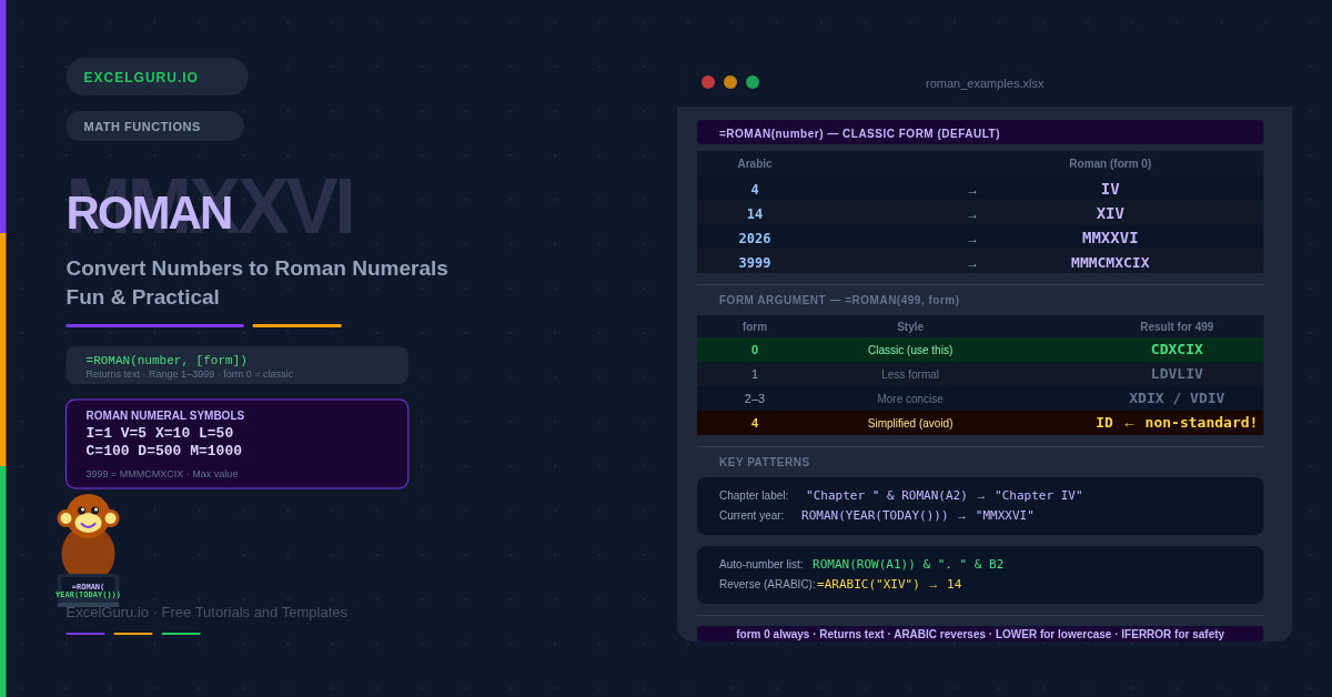
The form argument selects the convention used for the output. Form 0 applies the strict classical system you see in textbooks. Forms 1 through 4 introduce progressive simplifications — non-standard shorthand forms that produce shorter strings. Most users need form 0 only. The simplified forms are mainly useful for decorative or space-constrained contexts.
| Form | Style name | ROMAN(499, form) | ROMAN(1999, form) |
|---|---|---|---|
| 0 | Classic (default) | CDXCIX | MCMXCIX |
| 1 | Less formal | LDVLIV | MLMVLIV |
| 2 | More concise | XDIX | MXMIX |
| 3 | Concise | VDIV | MVMIV |
| 4 | Simplified | ID | MIM |
Notice how form 4 compresses 499 from six characters (CDXCIX) to two (ID). However, forms 1 through 4 use subtraction patterns that classical Roman numeral conventions do not recognise. Consequently, use form 0 for any document where the reader expects traditional notation.
Quick Reference — Common Roman Numeral Conversions
The table below shows frequently needed values. Each appears exactly as ROMAN(number, 0) returns it.
| Arabic | Roman | Arabic | Roman | Arabic | Roman |
|---|---|---|---|---|---|
| 1 | I | 10 | X | 100 | C |
| 4 | IV | 40 | XL | 400 | CD |
| 5 | V | 50 | L | 500 | D |
| 9 | IX | 90 | XC | 900 | CM |
| 2026 | MMXXVI | 3999 | MMMCMXCIX | 1000 | M |
Examples 1–4: Core Conversion Patterns
The simplest use is passing a cell reference directly to ROMAN. The function converts the integer part of the number and returns a text string. Decimal values are truncated, not rounded — so 4.9 becomes 4 (IV), not 5 (V).
Concatenating ROMAN with a text prefix creates formatted chapter or section labels automatically. The label updates whenever the source number changes, making it ideal for dynamically ordered documents where sections are renumbered frequently.
Nesting YEAR(TODAY()) inside ROMAN produces the current year as a Roman numeral. It updates automatically each time the workbook recalculates — ideal for copyright notices and report footers.
ROMAN returns #VALUE! for zero, negative numbers, numbers above 3999, and non-numeric input. In shared workbooks or templates where users enter numbers directly, IFERROR prevents these errors from disrupting the layout.
Examples 5–8: Creative and Advanced Uses
Styling, Reversing, and Combining
Academic and publishing conventions often use lowercase Roman numerals (i, ii, iii, iv) for front matter — prefaces, tables of contents, and acknowledgements. ROMAN always returns uppercase. Wrapping it in LOWER() converts the output to the lowercase style.
Using the ROW function as the input to ROMAN generates sequential Roman numerals automatically — no manual numbering required. Consequently, inserting or deleting rows in a list renumbers all subsequent items instantly without any formula editing.
ROMAN converts numbers to text. ARABIC reverses this — it converts a Roman numeral text string back to an Arabic number. This pairing is essential when you need to calculate with Roman numerals. Specifically, it helps with imported historical data or content where the format cannot be changed.
Edition numbers for recurring events often use Roman numerals — Super Bowl LVIII, the Paris 2024 Olympiad, wedding anniversaries. ROMAN makes this trivially easy for any event table, producing the correct numeral for each edition without manual lookup or typing.
Common ROMAN Issues and How to Fix Them
#VALUE! — number is out of range or invalid
ROMAN returns #VALUE! for four reasons: the number is zero, the number is negative, the number exceeds 3999, or the input is text rather than a number. Check the source cell with ISNUMBER(A2) — if it returns FALSE, the cell holds text-formatted numbers. Use VALUE(A2) to convert before passing to ROMAN. Additionally, wrap the formula in IFERROR to prevent the error from appearing in the output cell.
Decimal numbers produce unexpected output
ROMAN truncates decimals without rounding. A value of 4.9 returns "IV" (4), not "V" (5). If the source data has decimals and you want the nearest whole number, wrap in ROUND before ROMAN: =ROMAN(ROUND(A2, 0)). Alternatively, use INT to always round down: =ROMAN(INT(A2)).
ROMAN result does not match expected classical notation
If the form argument is set to 1–4, the output uses non-classical abbreviations that look different from standard Roman numerals. For example, form 4 converts 499 to "ID" instead of "CDXCIX". Always use form 0 (or omit the argument) for conventionally correct output. Additionally, verify that the form argument cell does not contain a non-zero value from a previous formula.
Frequently Asked Questions
-
What does the ROMAN function do in Excel?+ROMAN converts a positive whole number between 1 and 3999 into its Roman numeral equivalent as a text string. For example, =ROMAN(14) returns "XIV" and =ROMAN(2026) returns "MMXXVI". The result is always text — not a number — so it cannot be used in arithmetic directly. An optional form argument (0–4) controls the notation style, where 0 produces classical Roman numerals and 4 produces the most simplified version.
-
Why does ROMAN return #VALUE!?+ROMAN returns #VALUE! in four situations: the number is zero (Roman numerals have no zero), the number is negative, the number exceeds 3999, or the input is not a valid number. Wrap the formula in IFERROR to handle these gracefully: =IFERROR(ROMAN(A2), "Invalid"). Alternatively, use an IF guard to validate the range before converting: =IF(AND(A2>=1, A2<=3999), ROMAN(A2), "Enter 1–3999").
-
How do I convert Roman numerals back to numbers in Excel?+Use the ARABIC function — it is the exact reverse of ROMAN. =ARABIC("XIV") returns 14, and =ARABIC("MMXXVI") returns 2026. ARABIC also works on cell references: =ARABIC(A2) converts the Roman numeral text in A2 to a number. This is particularly useful when you need to sum or compare Roman numerals from imported historical data. ARABIC is available in Excel 2013 and later versions.
More Questions About ROMAN
-
How do I display Roman numerals in lowercase?+ROMAN always returns uppercase letters. Wrap the formula in LOWER() to convert the result to lowercase: =LOWER(ROMAN(A2)) returns "iv" for 4, "xii" for 12, and "mmxxvi" for 2026. Lowercase Roman numerals are conventional for book front matter — prefaces, acknowledgements, and tables of contents — where section numbers appear as i, ii, iii.
-
What is the highest number ROMAN can convert?+The maximum is 3999, which returns "MMMCMXCIX". This limit follows the traditional Roman numeral system, which has no standard symbol above M (1000) for larger quantities. Numbers above 3999 return #VALUE!. For values above 3999, a common workaround is to concatenate: display "MMMMCXLVII" for 4147 by dividing the number into thousands and remainder parts. However, this produces a non-standard result that most readers would not recognise as valid Roman notation.
-
When should I use the form argument?+In almost all practical cases, omit the form argument (or set it to 0) to get classical Roman numerals. Forms 1 through 4 produce progressive abbreviations that deviate from the standard notation — "ID" for 499 instead of "CDXCIX". These simplified forms are not widely recognised and should not be used in formal documents. The only reasonable use for forms 1–4 is in decorative or space-constrained contexts where the exact classical form is less important than brevity.