You have a column of numbers and you need the standard deviation. Excel gives you two main choices: STDEV.S and STDEV.P. Most people pick one and hope it is right. The difference is not cosmetic — it changes the result, and the wrong choice can produce misleading conclusions in quality control, financial analysis, and scientific reporting. This guide explains exactly when to use each function and why.
Standard deviation measures how spread out your data is. Specifically, it quantifies average distance from the mean. A low standard deviation means values cluster tightly around the mean. A high standard deviation means they spread widely. The two Excel functions produce different results because they divide by different denominators: STDEV.S divides by n−1 (the sample size minus one), while STDEV.P divides by n (the total count). This single difference has a meaningful statistical justification.
What Is Standard Deviation?
Standard deviation is the average distance between each data point and the mean. It is expressed in the same units as the original data, which makes it directly interpretable. For example, a standard deviation of £500 on a salary dataset means most salaries are within £500 of the average. A standard deviation of £15,000 indicates far greater variation.
The calculation involves four steps, and the distinction between the two functions appears in step four. First, find the mean. Second, subtract the mean from each value and square the result. Third, sum all the squared differences. Fourth, divide by n or n−1 and take the square root. The only difference between STDEV.S and STDEV.P is in step four — and that difference is the entire subject of this article.
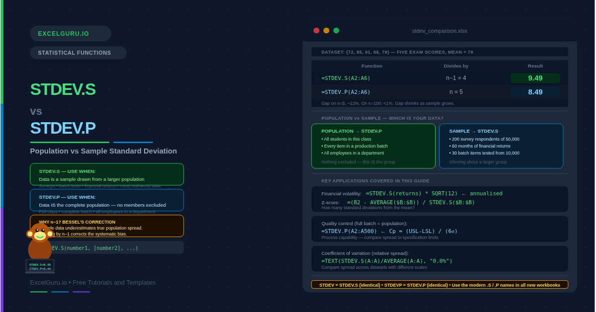
What Is the Difference Between STDEV.S and STDEV.P?
The distinction comes down to whether your data represents the entire group (a population) or just a subset (a sample). Use STDEV.S when your data is a sample drawn from a larger population. Use STDEV.P only when your data is the complete population — every single member, with none missing.
| Feature | STDEV.S | STDEV.P |
|---|---|---|
| Divides by | n−1 (Bessel’s correction) | n (total count) |
| Use when | Data is a sample from a larger population | Data IS the entire population |
| Result | Slightly larger — corrects for sampling bias | Slightly smaller — no bias correction |
| Legacy function | STDEV (identical results) | STDEVP (identical results) |
| Matches | R sd(), Python std(ddof=1), most statistical software defaults | R sd() with ddof=0, Python std(ddof=0), NumPy default |
| Most common choice | Yes — appropriate for most real-world analysis | Only when the dataset is truly complete |
Why Does n−1 Exist in STDEV.S?
Dividing by n−1 instead of n is called Bessel’s correction. This adjustment exists for a specific statistical reason. It exists because sample data tends to underestimate the true population spread. When you draw a sample, the values you observe are typically closer to the sample mean than to the true population mean. Dividing by a slightly smaller number (n−1) inflates the result just enough to correct for this systematic underestimation.
The effect is most pronounced on small samples. For instance, on n=5 the result increases by about 12%. For a sample of five values, dividing by 4 instead of 5 increases the result by about 12%. For a sample of 100 values, the difference is less than 1%. Consequently, on large datasets STDEV.S and STDEV.P produce nearly identical results. The choice still matters for correctness, but the numerical impact shrinks as n grows.
What Is the Syntax for Both Functions?
| Argument | Required? | What it does |
|---|---|---|
| number1 | Required | The first number, range, or array. Typically a cell range like A2:A100. Text and logical values are ignored. Zeros are included. |
| number2, ... | Optional | Additional numbers or ranges. Up to 255 arguments total. All values are pooled before the standard deviation is calculated. |
Examples 1–4: Core Standard Deviation Calculations
The best way to see the difference is to run both functions on the same small dataset. With only five values, the gap between STDEV.S and STDEV.P is clearly visible. As n grows, the gap narrows. This example uses exam scores from five students.
In manufacturing, a production batch is the entire population. Specifically, every item in the batch is measured. Every item in the batch is measured — nothing is left out. Because no sampling is involved, STDEV.P is correct here. The result feeds directly into process capability calculations such as Cp and Cpk, which compare the standard deviation to specification limits.
Consider a customer satisfaction survey that reaches 200 respondents from a customer base of 50,000. The 200 scores are a sample — not the full population. To draw valid conclusions about all 50,000 customers, use STDEV.S. The n−1 correction makes the estimate more conservative and reduces overconfidence when inferring from a subset to the whole.
Standard deviation is expressed in the same units as the data, which is useful for direct interpretation. This makes comparing standard deviations across different metrics difficult — a standard deviation of 10 means something very different for a dataset with a mean of 20 versus a mean of 10,000. The coefficient of variation (CV) solves this by expressing spread as a percentage of the mean.
Examples 5–8: Applied Scenarios
Finance, HR, and Academic Applications
In finance, standard deviation of returns is the standard measure of volatility. Furthermore, it is the denominator in the Sharpe ratio. Monthly or daily return data is a sample — a subset of all possible future returns. Consequently, STDEV.S is correct. To compare annual volatility across assets measured at different frequencies, multiply by the square root of the number of periods per year.
A compensation analyst reviewing salaries for one job grade typically has data for every employee in that grade. Consequently, the dataset is a population. That makes it a population, not a sample — so STDEV.P is correct. However, if the goal is to benchmark against an external salary survey that used a sample of companies, switch to STDEV.S. The choice depends on whether the data represents the full group or a subset.
A z-score tells you how many standard deviations a specific value sits above or below the mean. It is therefore a dimensionless measure of relative position. It standardises values from different scales onto a single comparable axis. Use the same function for the z-score denominator as you would for reporting the standard deviation — STDEV.S for samples, STDEV.P for populations.
A rolling standard deviation calculates the spread over a moving window of recent periods, which is useful for tracking change over time. This is widely used in financial dashboards to show whether volatility is increasing or decreasing over time. Each row looks back a fixed number of periods — for example, the last 12 months. Because each window is a sample of recent data, STDEV.S is appropriate.
Common Issues and How to Fix Them
Which function should I use if I am not sure?
Use STDEV.S as your default in almost every scenario. Most datasets in business, finance, and research are samples — they represent a subset drawn from a larger group. The n−1 correction in STDEV.S produces a more conservative and statistically unbiased estimate. Use STDEV.P only when you are certain the data covers every member of the population with no omissions.
STDEV gives a different result to what I expect
First, check whether the range contains blank cells, text values, or zeros that should not be included. STDEV.S ignores text and blanks but includes zeros. Additionally, confirm whether your data uses STDEV.S or STDEV.P relative to what external tools report. R’s sd() function uses n−1 (matching STDEV.S). Python’s NumPy std() uses n by default (matching STDEV.P), while Pandas std() uses n−1 (matching STDEV.S).
The standard deviation is zero
A zero result means every value in the range is identical. Additionally, check that the correct range is referenced. Check that the correct range is referenced and that the data has not been accidentally rounded or truncated to remove variation. STDEV.S with only one value returns a #DIV/0! error because dividing by n−1 = 0 is undefined. STDEV.P with one value returns zero. Both are correct for their respective scenarios.
Frequently Asked Questions
-
What is the difference between STDEV.S and STDEV.P?+STDEV.S calculates the sample standard deviation by dividing by n−1. STDEV.P calculates the population standard deviation by dividing by n. Use STDEV.S when your data is a sample drawn from a larger population — a survey, a batch sample, or any subset. Use STDEV.P only when your data represents the entire population with no values excluded. STDEV.S is correct for most real-world datasets. The difference in results is most significant on small samples — on large datasets the two values converge.
-
Why does STDEV.S divide by n−1 instead of n?+This is Bessel’s correction. Sample data tends to cluster closer to the sample mean than to the true population mean. As a result, dividing by n systematically underestimates the true population variance. Dividing by n−1 inflates the result just enough to correct for this bias. The correction produces an unbiased estimator of the population variance when the data is a random sample — which is almost always the case in practice. For large n, the difference between n and n−1 becomes negligible.
-
Is STDEV the same as STDEV.S?+Yes — STDEV and STDEV.S produce identical results. STDEV is the legacy function from Excel versions before 2010. Microsoft introduced STDEV.S (and STDEV.P) to make the sample vs. population distinction explicit in the function name. STDEV remains available for backward compatibility but STDEV.S is recommended for all new workbooks. Similarly, STDEVP and STDEV.P are identical — use STDEV.P going forward.
More Questions About Standard Deviation
-
When should I use STDEV.P instead of STDEV.S?+Use STDEV.P specifically when your dataset IS the entire population — not a sample drawn from it. Practical examples include: all students in a single class (not a sample of students from all classes), every item produced in a specific manufacturing batch, all employees in a department, or all transactions in a closed fiscal period where nothing was excluded. If even one member of the population was not measured or included, the data is a sample and STDEV.S is correct.
-
What is the difference between STDEV.S and STDEV.A?+STDEV.A is the “A” (all values) variant of the sample standard deviation. It differs from STDEV.S in how it handles text and logical values. STDEV.S ignores text strings and TRUE/FALSE values in the range entirely. STDEV.A counts logical TRUE as 1 and FALSE as 0, and converts text strings to 0. For most numeric datasets these functions return the same result. Use STDEV.A only when you specifically need logical values or text-as-zero included in the calculation.
-
How do I calculate standard deviation for a filtered or conditional range?+STDEV.S and STDEV.P do not support conditional filtering natively — they operate on a fixed range. For conditional standard deviation, combine them with IF in an array formula. In Excel 365, enter =STDEV.S(IF(B2:B100="North", A2:A100)) normally. In Excel 2019 and earlier, press Ctrl+Shift+Enter to confirm it as an array formula. Alternatively, use a helper column to filter the values and then run STDEV.S on the filtered column.