Filter a table and SUM keeps counting every row — including the hidden ones. Use SUBTOTAL instead and the total updates the moment a filter is applied. SUBTOTAL is the only native Excel function that automatically ignores filtered-out rows. It also optionally ignores manually hidden rows, and it skips nested SUBTOTAL calls so you can safely place it inside a table without double-counting. These three behaviours together make SUBTOTAL the indispensable function for any report built on filtered or structured data.
This guide covers every function number, the difference between the 1–11 and 101–111 ranges, and eight practical examples. You will learn how to build filter-aware totals, counts, and averages, create a running subtotal that ignores hidden rows, detect which rows are visible, and combine SUBTOTAL with structured table references. Each example also shows the equivalent using AGGREGATE — the modern upgrade that handles errors and offers more functions.
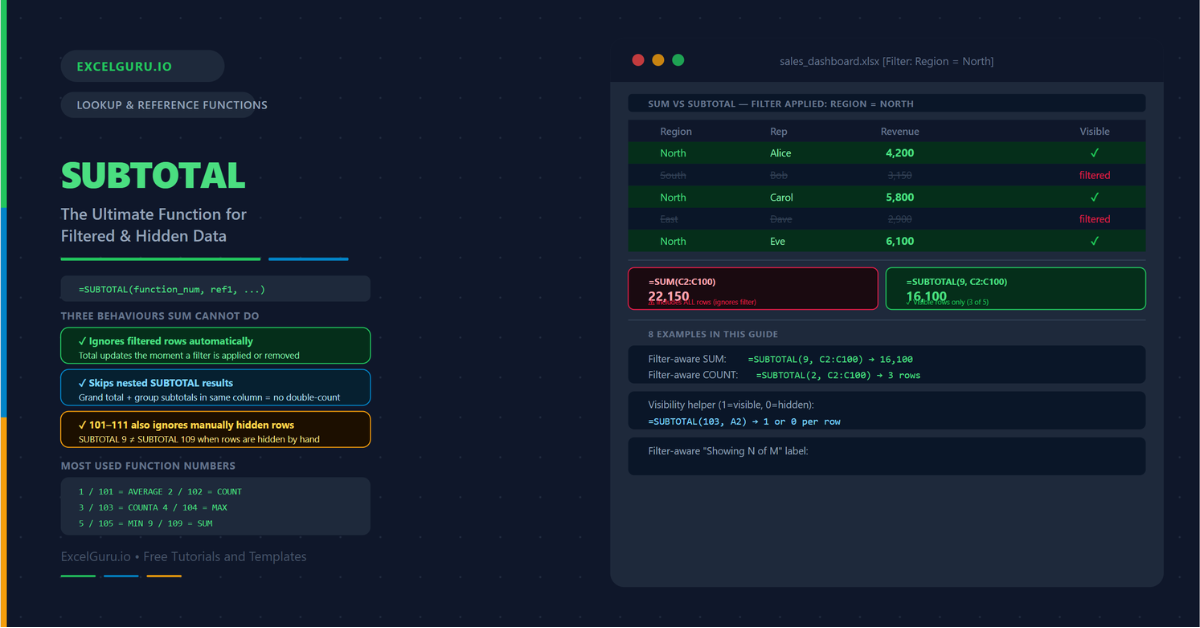
What Makes SUBTOTAL Different from SUM?
SUM adds every cell in its range, whether visible or not. Filter the table and SUM does not change. SUBTOTAL, by contrast, operates only on the visible rows. It recalculates automatically whenever a filter changes, when rows are hidden manually, or when the display changes for any reason. This makes SUBTOTAL the correct choice for any total that should reflect the current filtered view rather than the full dataset.
SUBTOTAL also has a second key behaviour: it ignores other SUBTOTAL results nested inside its range. Specifically, if column B contains multiple SUBTOTAL formulas — one per group — and a grand total SUBTOTAL at the bottom references all of column B, the grand total does not double-count the group subtotals. This makes SUBTOTAL safe to use in nested grouping structures without needing to carefully exclude the subtotal rows from the grand total range.
What Is the SUBTOTAL Syntax?
| Argument | Required? | What it does |
|---|---|---|
| function_num | Required | A number from 1–11 or 101–111 that specifies the aggregation type. Numbers 1–11 ignore filtered rows but include manually hidden rows. Numbers 101–111 ignore both filtered rows and manually hidden rows. |
| ref1 | Required | The first range of values to aggregate. Accepts up to 254 additional range arguments (ref2, ref3, ...) for aggregating multiple non-contiguous ranges. |
What Are the SUBTOTAL Function Numbers?
The function_num argument determines which aggregation SUBTOTAL performs. Numbers 1–11 include manually hidden rows but ignore filtered rows. Numbers 101–111 ignore both — manually hidden rows and filtered rows. In practice, the 1–11 range is used in most formula-based totals. The 101–111 range is more appropriate when rows are hidden by hand (not by filter) and the total should exclude them.
| 1–11 | 101–111 | Function | Equivalent to |
|---|---|---|---|
| 1 | 101 | AVERAGE | =AVERAGE of visible rows |
| 2 | 102 | COUNT | =COUNT of visible rows (numbers only) |
| 3 | 103 | COUNTA | =COUNTA of visible rows (non-empty) |
| 4 | 104 | MAX | =MAX of visible rows |
| 5 | 105 | MIN | =MIN of visible rows |
| 6 | 106 | PRODUCT | =PRODUCT of visible rows |
| 7 | 107 | STDEV | =STDEV of visible rows |
| 8 | 108 | STDEVP | =STDEVP of visible rows |
| 9 | 109 | SUM | =SUM of visible rows |
| 10 | 110 | VAR | =VAR of visible rows |
| 11 | 111 | VARP | =VARP of visible rows |
Examples 1–4: Core SUBTOTAL Patterns
The most common use is replacing SUM, COUNT, and AVERAGE with SUBTOTAL equivalents in a totals row below a filtered table. When a filter is applied, the SUBTOTAL values update immediately to reflect only the visible rows. The SUM equivalent is function 9, COUNT is function 2, and AVERAGE is function 1.
In grouped reports, each group has its own subtotal row and a grand total at the bottom covers the entire column. If you use SUM for both levels, the grand total double-counts the group subtotals. SUBTOTAL prevents this — it automatically skips any SUBTOTAL result nested inside its range. Consequently, the grand total SUBTOTAL can safely reference the entire column including the subtotal rows.
Function numbers 1–11 respect AutoFilter but include manually hidden rows. Function numbers 101–111 exclude both filtered and manually hidden rows. This distinction matters when rows are hidden via Home → Format → Hide Rows or via grouping and collapsing. In those cases, function 9 still counts the hidden rows while function 109 ignores them.
SUBTOTAL with function 3 (COUNTA) on a single row returns 1 if that row is visible and 0 if it is filtered out. This per-row indicator is the foundation of many filter-aware formulas. Specifically, you can use it to build a sequential row number that resets with the filter, flag visible rows for conditional formatting, or feed it into SUMPRODUCT for conditional aggregation on visible rows.
Examples 5–8: Applied SUBTOTAL Techniques
Excel Tables, AGGREGATE, and Dynamic Dashboards
When you format data as an Excel Table (Ctrl+T), turning on the Total Row automatically inserts SUBTOTAL formulas. The Total Row dropdown lets you choose SUM, COUNT, AVERAGE, and so on — and Excel uses the appropriate SUBTOTAL function number behind the scenes. Additionally, table references adjust automatically when new rows are added, so the SUBTOTAL range never needs manual updating.
AGGREGATE is the extended version of SUBTOTAL, available from Excel 2010. It adds two major capabilities that SUBTOTAL lacks. First, it can ignore error values in the range — so #DIV/0! or #VALUE! in one cell does not break the total. Second, it supports additional functions that SUBTOTAL does not include: LARGE, SMALL, MEDIAN, PERCENTILE, and RANK. Furthermore, AGGREGATE accepts an options argument that controls exactly which rows to ignore.
A management dashboard built on SUBTOTAL updates all KPI cells the moment a slicer or filter changes. Each metric references the same table column with a different function number. Adding a progress bar or conditional formatting to the KPI cells makes the changes immediately visible. No VBA, no Power Query refresh — the dashboard is entirely formula-driven.
SUMIF and COUNTIF do not respect filters. They count and sum all matching rows, including filtered-out ones. Consequently, combining a filter with SUMIF gives misleading results — the SUMIF total does not change when the filter changes. Two approaches solve this problem: SUMPRODUCT with the SUBTOTAL(103) visibility indicator, or using AGGREGATE for the aggregation and applying the condition separately.
Common Issues and How to Fix Them
SUBTOTAL does not change when I apply a filter
SUBTOTAL only responds to AutoFilter (Data → Filter or Table filters). It does not respond to manual colour-based filtering, slicer-only filtering on ranges that are not tables, or filtering applied via VBA on a different sheet. If the filter is an AutoFilter and SUBTOTAL still does not update, check that Automatic Calculation is enabled: Formulas → Calculation Options → Automatic. Additionally, confirm the SUBTOTAL range overlaps with the filtered rows — a range that accidentally excludes some rows will not change even if those rows are filtered.
SUBTOTAL and SUM give different results even without a filter
SUBTOTAL skips nested SUBTOTAL values inside its range. If the range contains subtotal rows from a grouped structure, SUBTOTAL deliberately excludes them — this is the intended behaviour for grand totals. If you need SUM to include all values including other SUBTOTAL results, use SUM instead. Conversely, if the results differ and you did not expect them to, inspect the range for hidden SUBTOTAL rows that SUBTOTAL is skipping.
SUBTOTAL with errors — the result shows #VALUE! or #DIV/0!
SUBTOTAL propagates errors from the cells in its range. If one cell in the range contains #DIV/0!, #VALUE!, or any other error, SUBTOTAL returns that error. The fix is to switch to AGGREGATE with options = 6 (ignore errors) or options = 7 (ignore hidden rows and errors). For example, =AGGREGATE(9, 7, C2:C100) sums visible rows and skips any error cells without returning an error itself.
Frequently Asked Questions
-
What is the SUBTOTAL function in Excel?+SUBTOTAL is a multi-purpose aggregation function that operates only on visible (non-filtered) rows. It accepts a function number (1–11 or 101–111) that specifies whether to SUM, COUNT, AVERAGE, MAX, MIN, or apply other operations. Unlike SUM or AVERAGE, SUBTOTAL automatically ignores rows that have been hidden by AutoFilter. It also skips any other SUBTOTAL results nested inside its range, making it safe for grouped reports with subtotals and grand totals. In Excel Tables, the Total Row uses SUBTOTAL by default.
-
What is the difference between SUBTOTAL 9 and SUBTOTAL 109?+Both calculate SUM and both ignore rows hidden by AutoFilter. The difference is manual hiding. SUBTOTAL 9 includes rows that were hidden manually via Home → Format → Hide Rows or by collapsing a group outline. SUBTOTAL 109 excludes those manually hidden rows as well. For most filtered tables, the two produce identical results because rows are hidden by filter, not manually. Use 109 when rows are hidden by grouping or outline and you want the total to reflect only the displayed rows.
-
Why does SUMIF not work with filtered data?+SUMIF evaluates all rows in its range regardless of filter status. It has no awareness of which rows are currently visible. Consequently, applying a filter does not change the SUMIF result. To get a filter-aware conditional sum, use SUMPRODUCT combined with a SUBTOTAL(103) visibility helper column. The helper column returns 1 for visible rows and 0 for filtered-out rows. Multiplying SUMPRODUCT by that helper effectively limits the sum to visible rows only. Alternatively, AGGREGATE handles many aggregations on visible rows, though it does not support condition-based filtering natively.
More Questions About SUBTOTAL
-
What is the difference between SUBTOTAL and AGGREGATE?+SUBTOTAL supports 11 aggregation functions and cannot handle errors in the range. AGGREGATE supports 19 functions — including MEDIAN, LARGE, SMALL, PERCENTILE, and RANK — and can optionally ignore error values. AGGREGATE also offers more granular control over which rows to ignore via the options argument. The trade-off is availability: SUBTOTAL works in all Excel versions and Google Sheets, while AGGREGATE requires Excel 2010 or later and does not work in Google Sheets. For most everyday filter-aware totals, SUBTOTAL is sufficient. Use AGGREGATE when you need error tolerance or functions beyond SUBTOTAL’s 11.
-
Can SUBTOTAL work with multiple ranges?+Yes. SUBTOTAL accepts up to 255 range arguments: =SUBTOTAL(9, A2:A50, C2:C50, E2:E50). This sums all three columns counting only visible rows in each. However, all ranges must be on the same sheet — SUBTOTAL cannot span multiple worksheets. The multiple-range capability is useful when non-contiguous columns need to be aggregated together in one formula. Note that the ranges should not overlap, as overlapping ranges cause values in the overlap to be counted multiple times.
-
Does SUBTOTAL work in Google Sheets?+Yes, SUBTOTAL works in Google Sheets with the same function numbers and syntax as Excel. It responds to filters applied via Data → Create a Filter. However, AGGREGATE is not available in Google Sheets — it is an Excel-only function. If you need median, percentile, or error-ignoring behaviour in Google Sheets with filter awareness, the SUBTOTAL(103) visibility helper combined with SUMPRODUCT is the most reliable workaround.