FILTER returns everything that matches. SORT returns everything reordered. But sometimes you only want the first five rows, or everything except the last three, or a specific middle slice. Before Excel 365 introduced TAKE and DROP, extracting a partial array required OFFSET, INDEX, or a complex SEQUENCE-based construction. Now two functions handle every slicing scenario cleanly. TAKE returns a specified number of rows or columns from the beginning or end of an array. DROP removes a specified number from either end and returns the rest.
This guide covers both functions in full, the negative-number shortcut for working from the end of an array, and six practical examples. You will learn how to extract top-N and bottom-N rows, remove headers or footers from a dynamic array, combine TAKE and DROP for a middle slice, and chain these functions with SORT, FILTER, and UNIQUE for precise array control. Each example also shows the pre-TAKE workaround so you can see exactly what TAKE replaces.
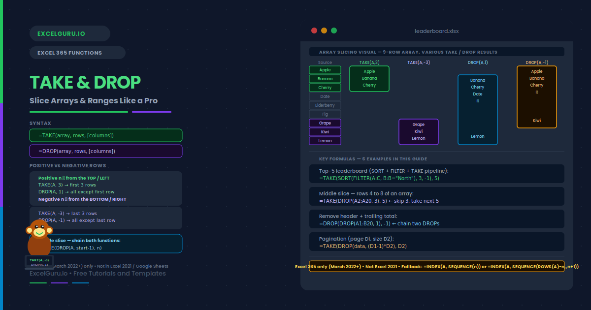
What Are TAKE and DROP?
TAKE and DROP are complementary array-slicing functions. TAKE keeps a portion of an array. DROP removes a portion and returns the remainder. Together they cover every scenario where you need a subset of an array rather than the whole thing. Positive row/column numbers work from the top-left corner. Negative numbers work from the bottom-right corner. This negative-number shortcut is the key to extracting the last N rows without knowing the total length of the array.
Both functions accept two-dimensional arrays, which means they work on tables as well as single columns. Specifying both rows and columns lets you extract a rectangular sub-table from a larger range. Omitting the columns argument slices by row only and returns all columns. Similarly, omitting the rows argument slices by column only.
What Is the TAKE and DROP Syntax?
| Argument | TAKE behaviour | DROP behaviour |
|---|---|---|
| array | The source array or range. Can be a cell range, named range, or the result of any spilling function. | |
| rows (positive) | Keep the first n rows | Remove the first n rows, return the rest |
| rows (negative) | Keep the last n rows | Remove the last n rows, return the rest |
| columns (positive) | Keep the first n columns | Remove the first n columns, return the rest |
| columns (negative) | Keep the last n columns | Remove the last n columns, return the rest |
| rows = 0 | Returns empty (use with caution) | Returns entire array (removes nothing) |
How Do TAKE and DROP Compare to Older Methods?
Before TAKE and DROP, extracting a slice required INDEX with SEQUENCE or OFFSET — both verbose and fragile with dynamic arrays. The table below shows each slicing scenario and the old vs new formula approach.
| Scenario | Old approach | TAKE / DROP approach |
|---|---|---|
| First 5 rows | =INDEX(A:A, SEQUENCE(5)) | =TAKE(A2:A100, 5) |
| Last 5 rows | =INDEX(A:A, ROWS(A2:A100)-4+SEQUENCE(5)) | =TAKE(A2:A100, -5) |
| Skip first row | =INDEX(A:A, SEQUENCE(ROWS(A2:A100)-1,,2)) | =DROP(A2:A100, 1) |
| Skip last row | =INDEX(A:A, SEQUENCE(ROWS(A2:A100)-1)) | =DROP(A2:A100, -1) |
| Middle slice (rows 3–7) | =INDEX(A:A, SEQUENCE(5,,3)) | =TAKE(DROP(A2:A100, 2), 5) |
Examples 1–4: Core TAKE and DROP Patterns
The most common use is extracting a fixed number of rows from the top or bottom of a data column. TAKE with a positive number returns from the top. TAKE with a negative number returns from the bottom. Both work identically whether the source is a static range or the spilled result of SORT or FILTER.
DROP is particularly useful when a dynamic array includes rows you want to exclude. The most common case is removing a header row from a spilled result. Another frequent use is stripping a running total or grand total row that appears at the bottom of a dynamic output. DROP handles both without requiring you to know the total row count.
Neither TAKE nor DROP alone can extract a middle segment — rows 4 through 8 from a 20-row array, for example. Chaining the two functions solves this. First, DROP removes the rows before the desired segment. Then TAKE keeps only as many rows as needed from the remaining array. This pattern replaces the old INDEX+SEQUENCE middle-slice formula with a clean, readable two-function chain.
TAKE and DROP both accept a columns argument as well as rows. This enables two-dimensional slicing — extracting a rectangular block from a larger table. Specifying both rows and columns lets you return exactly the columns you need from the top N rows, or remove the first column while also removing the last row. This is particularly useful for reshaping structured table outputs from FILTER or SORT.
Examples 5 and 6: Applied TAKE and DROP
Pipeline Patterns and Dynamic Reports
TAKE becomes most powerful when chained at the end of a FILTER and SORT pipeline. The pattern is: FILTER to select the relevant rows, SORT to put them in the desired order, and TAKE to limit the output to exactly the number of rows you want to display. This produces a self-updating leaderboard or top-N report that responds to data changes without any manual adjustment.
TAKE and DROP together enable in-worksheet pagination. A page number input cell controls which set of N rows is displayed. Page 1 shows rows 1–10, page 2 shows rows 11–20, and so on. This pattern is useful for dashboards where space is limited and results need to be browsed in chunks rather than displayed all at once.
Common Issues and How to Fix Them
TAKE or DROP is not available in my Excel version
TAKE and DROP require Excel 365, specifically the March 2022 channel release or later. They are not in Excel 2021, 2019, or Google Sheets. To check your version, go to File → Account → About Excel. In older versions, use =INDEX(array, SEQUENCE(n)) for TAKE and =INDEX(array, SEQUENCE(ROWS(array)-n,,n+1)) for a DROP equivalent. Both require Ctrl+Shift+Enter in Excel 2019 and earlier.
TAKE returns a #CALC! error
#CALC! from TAKE means the rows or columns argument exceeds the size of the array. For example, TAKE(A2:A5, 10) asks for 10 rows from a 4-row array. TAKE does not truncate silently — it errors. Consequently, wrap the n argument with MIN to cap it at the actual array size: =TAKE(A2:A100, MIN(5, ROWS(A2:A100))). This returns up to 5 rows and fewer if the array is smaller.
DROP with rows = 0 behaves unexpectedly
Passing rows = 0 to DROP returns the entire array unchanged — it removes nothing. This is the intended behaviour and is useful when the skip amount is calculated dynamically and happens to evaluate to zero. However, passing rows = 0 to TAKE returns an empty array, which causes a #CALC! error in most contexts. Always test the formula when a dynamic n argument might evaluate to zero, and add an IF guard if needed: =IF(n=0, array, TAKE(array, n)).
Frequently Asked Questions
-
What does the TAKE function do in Excel?+TAKE extracts a specified number of rows or columns from the beginning or end of an array. Pass a positive number to take from the top or left. Pass a negative number to take from the bottom or right. For example, =TAKE(A2:A100, 5) returns the first 5 rows, and =TAKE(A2:A100, -5) returns the last 5 rows. TAKE can also work on two dimensions: =TAKE(A2:D100, 5, 2) returns the first 5 rows and first 2 columns. The function is available in Excel 365 from March 2022 onward. It spills automatically and does not require array entry.
-
What does the DROP function do in Excel?+DROP removes a specified number of rows or columns from an array and returns the remainder. A positive number removes from the top or left. A negative number removes from the bottom or right. For example, =DROP(A2:A100, 3) removes the first 3 rows and returns rows 4–100, and =DROP(A2:A100, -1) removes the last row and returns everything else. This is the complement of TAKE — where TAKE keeps a portion, DROP discards a portion. Combining TAKE and DROP enables middle-slice extraction and pagination patterns.
-
How do I extract the last N rows without knowing the total row count?+Use TAKE with a negative number: =TAKE(A2:A100, -5) returns the last 5 rows regardless of how many total rows are in the array. The negative sign means "count from the bottom." This works even when the array is the result of a FILTER or SORT that returns a variable number of rows — you always get the last N rows of whatever the dynamic result contains. Similarly, =DROP(A2:A100, -3) removes the last 3 rows and returns everything else, again without needing to know the total count.
More Questions About TAKE and DROP
-
Can I use TAKE and DROP on the result of FILTER?+Yes — this is one of the most common and powerful combinations. Pass FILTER (or SORT(FILTER(...))) as the first argument of TAKE or DROP. For example, =TAKE(SORT(FILTER(A2:C100, B2:B100="North"), 3, -1), 5) returns the top 5 rows from the filtered-and-sorted result. Because TAKE receives the full dynamic array from FILTER, it always operates on the correct set of rows regardless of how many rows FILTER returns. This makes TAKE the standard method for top-N leaderboards and paginated reports in Excel 365.
-
How do I extract a middle slice (rows 4 to 8) using TAKE and DROP?+Chain DROP and TAKE: first DROP to remove the rows before your target, then TAKE to keep only the rows you want. To extract rows 4–8 of an array: =TAKE(DROP(A2:A20, 3), 5). The DROP(array, 3) removes the first 3 rows, leaving rows 4 onward as the new first row. Then TAKE(..., 5) keeps the first 5 rows of that result, giving you rows 4–8 of the original. For a dynamic version with configurable start and length, use cell references for the arguments: =TAKE(DROP(A2:A20, D1-1), D2), where D1 is the start row and D2 is the number of rows to extract.
-
What is the difference between TAKE and INDEX for extracting rows?+INDEX with SEQUENCE was the pre-TAKE workaround for extracting a fixed number of rows. For example, =INDEX(A2:A100, SEQUENCE(5)) returns the first 5 rows, similar to =TAKE(A2:A100, 5). TAKE is simpler to write and read, handles negative indexing naturally (last N rows), and works directly on dynamic array results without requiring a separate SEQUENCE call. The key limitation is availability — INDEX+SEQUENCE works in all Excel versions with dynamic array support (Excel 365 and 2021), while TAKE requires Excel 365 specifically. For workbooks that need to run in Excel 2021, use INDEX+SEQUENCE as the more compatible alternative.