TOCOL & TOROW in Excel: Flatten Ranges into Single Columns or Rows

TOCOL and TOROW functions in Excel 365 — showing a 3×3 grid flattened three ways: TOCOL with scan=FALSE reading row-by-row producing 1,2,3,4,5,6,7,8,9 in a green column, TOCOL with scan=TRUE reading column-by-column producing 1,4,7,2,5,8,3,6,9 in a teal column, and TOROW producing a horizontal row in indigo, with key formulas for cross-column UNIQUE deduplication, WRAPROWS pipeline, multi-sheet master list, and tag grid TEXTJOIN.
FILTER returns a table. WRAPROWS needs a column. UNIQUE works best on a flat list. TOCOL is the missing link — it flattens any 2D range into a single column in one formula. TOROW does the same into a single row. This guide covers eight examples: basic flattening with row-by-row vs column-by-column scan direction, all four ignore values for removing blanks and errors, stacking multiple columns for cross-column UNIQUE deduplication, converting rows to columns for SORT, the TOCOL+WRAPROWS flatten-then-reshape pipeline, building a master list from multiple sheets using VSTACK+TOCOL, feeding a 2D tag grid into TEXTJOIN, and deduplicating values across five columns for a dynamic dropdown source.

FILTER returns a multi-column table. WRAPROWS needs a single column. UNIQUE produces a column you want to feed into TEXTJOIN. These transitions — from 2D array to flat vector — are the domain of TOCOL and TOROW. TOCOL flattens any range or array into a single column. TOROW does the same into a single row. Both give you control over which cells to include and the reading direction (row-by-row or column-by-column). They are the essential pre-processing step before functions that require 1D input.

This guide covers both functions fully with eight practical examples. You will learn how to flatten a table for UNIQUE deduplication and stack multiple columns. You will also convert rows to columns for SORT, clean blanks and errors, and build a master list from multiple named ranges. Each example also shows the old workaround so you see exactly what TOCOL and TOROW replace.

Availability: TOCOL and TOROW are available in Excel 365 only (August 2022 or later). They are not in Excel 2021, 2019, or Google Sheets. For older versions, use OFFSET+INDIRECT combinations or old-style CSE array formulas. Neither TOCOL nor TOROW requires Ctrl+Shift+Enter — both spill automatically.

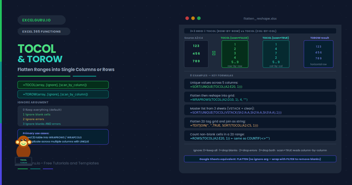
What Are TOCOL and TOROW?

TOCOL reads a 2D range and outputs a single vertical column. TOROW does the same but outputs a single horizontal row. Both functions flatten the source array in a specified reading order and can optionally filter out blanks, errors, or both. The ignore argument controls what to exclude before flattening.

The scan argument controls the reading direction. By default, both functions read left to right across each row, then down to the next. Setting scan = TRUE switches to column-by-column reading: top to bottom, then right to the next column. Specifically, the scan direction determines the order of values in the output.

What Is the TOCOL and TOROW Syntax?

=TOCOL(array, [ignore], [scan_by_column]) =TOROW(array, [ignore], [scan_by_column])
ArgumentRequired?Description
arrayRequiredThe 2D or 1D range or array to flatten. Can be a cell range, named range, or any dynamic array expression.
ignoreOptional0 (default) = keep all values. 1 = ignore blanks. 2 = ignore errors. 3 = ignore both blanks and errors.
scan_by_columnOptionalFALSE (default) = read row-by-row (left-right, then down). TRUE = read column-by-column (top-bottom, then right). Determines the order of values in the output.
ignore argument quick reference: 0 = keep everything, 1 = drop blanks, 2 = drop errors, 3 = drop both. The most commonly used values are 1 (drop blanks) and 3 (drop both blanks and errors). Use 3 before passing a messy range to UNIQUE or WRAPROWS.

Examples 1–8: TOCOL and TOROW in Practice

1
Basic flatten — 2D range to single column or row

The core use is converting a multi-column range into a single column (or row) for further processing. TOCOL reads row-by-row by default — all values from row 1, then row 2, and so on. TOROW does the same but outputs horizontally. Both preserve the original values exactly.

A
B
C
TOCOL result (rows)
TOCOL result (cols)
1
2
3
1,2,3,4,5,6,7,8,9
1,4,7,2,5,8,3,6,9
4
5
6
(scan=FALSE, row-by-row)
(scan=TRUE, col-by-col)
7
8
9
A2:C4 = 3×3 grid {1,2,3;4,5,6;7,8,9}. TOCOL — flatten to a single column, row-by-row (default): =TOCOL(A2:C4) → {1;2;3;4;5;6;7;8;9} (reads left-to-right across each row) TOCOL — flatten column-by-column (scan = TRUE): Reads down column A, then B, then C. =TOCOL(A2:C4, 0, TRUE) → {1;4;7;2;5;8;3;6;9} (different order — column-by-column) TOROW — flatten to a single row: =TOROW(A2:C4) → {1,2,3,4,5,6,7,8,9} (same values, horizontal output)
2
Clean blanks and errors — use ignore to filter before flattening

The ignore argument removes unwanted values during the flatten operation. This is much cleaner than running IFERROR or filtering blanks after the fact. Specifically, ignore = 1 drops blank cells, ignore = 2 drops error cells, and ignore = 3 drops both. The remaining values are packed together in reading order without gaps.

A2:C4 = range with blanks and errors mixed in. E.g. {1, "", 3; #DIV/0!, 5, 6; 7, "", 9} ignore = 0 (default) — keep everything including blanks and errors: Result contains blanks and propagated errors. =TOCOL(A2:C4, 0) → {1; ""; 3; #DIV/0!; 5; 6; 7; ""; 9} (all values including blanks/errors) ignore = 1 — drop blank cells only: =TOCOL(A2:C4, 1) → {1; 3; #DIV/0!; 5; 6; 7; 9} (blanks removed, error kept) ignore = 2 — drop error cells only: =TOCOL(A2:C4, 2) → {1; ""; 3; 5; 6; 7; ""; 9} (error removed, blanks kept) ignore = 3 — drop both blanks and errors: Cleanest result for further processing. =TOCOL(A2:C4, 3) → {1; 3; 5; 6; 7; 9} (only valid, non-blank values remain)
3
Stack multiple columns — combine several columns into one

TOCOL on a multi-column range stacks all columns into a single list. This is the standard way to feed a 2D table into functions that require a 1D input, like UNIQUE for deduplication across multiple columns, or WRAPROWS for reshaping. Choosing scan = FALSE stacks columns left-to-right (rows first); scan = TRUE stacks column-by-column (columns first).

A2:C10 = 3 columns of product categories (each column may overlap the others). Goal: get a unique list of all categories from all three columns. Step 1: TOCOL flattens all three columns into one list (row-by-row): Ignore = 1 to skip blank cells in shorter columns. =TOCOL(A2:C10, 1) → Flat column with all values from A, B, C combined (blanks removed) Step 2: UNIQUE removes duplicates across all three source columns: =UNIQUE(=TOCOL(A2:C10, 1)) → Each distinct category exactly once, from all three columns Sort the unique list alphabetically: =SORT(UNIQUE(=TOCOL(A2:C10, 1))) → Distinct categories in A–Z order TOROW equivalent — unique values as a single row instead of column: =UNIQUE(=TOROW(A2:C10, 1), TRUE) → Distinct values as a horizontal row Note: UNIQUE with by_col=TRUE for a row-wise deduplication
4
Convert a row to a column — rotate 1D arrays for SORT and FILTER

Many functions work with columns but not rows, or the other way around. TOCOL on a single row converts it to a column. TOROW on a single column converts it to a row. This is a simpler alternative to TRANSPOSE in many situations, especially when combined with ignore to clean blanks at the same time.

A1:J1 = a single row of 10 values (header row or month names). Convert row to column (no blank cleaning needed): TOCOL on a single row is the clean alternative to TRANSPOSE. =TOCOL(A1:J1) → Same 10 values, now in a vertical column (J rows × 1 column) Compare: TRANSPOSE also works but is more verbose: =TRANSPOSE(A1:J1) → same result, but TOCOL is more self-documenting Convert column to row: A2:A20 = a vertical list. TOROW converts it horizontal. =TOROW(A2:A20) → Same 19 values, now in a single row Sort a row of values using SORT on the TOCOL result: SORT works on columns. Convert row to column, sort, convert back. =TOROW(SORT(=TOCOL(A1:J1))) → Values from A1:J1 sorted ascending, returned as a row

Examples 5–8: Advanced TOCOL and TOROW Patterns

5
TOCOL into WRAPROWS — flatten then reshape

WRAPROWS requires a 1D input. TOCOL is the standard way to flatten a multi-column table before passing it to WRAPROWS. This combination converts a 2D table into a flat list, then reshapes the list into a grid of specified width. The ignore argument additionally removes blanks during flattening so the resulting grid has no empty slots from sparse source data.

A2:D10 = a 4-column, 9-row table (36 values, possibly with some blanks). Goal: flatten all values (ignoring blanks) then wrap into a 4-column display grid. Step 1: TOCOL flattens and removes blanks (ignore = 1): Produces a compact list of all non-blank values. =TOCOL(A2:D10, 1) Step 2: WRAPROWS reshapes the flat list into rows of 4: Result is a grid matching the original column count. =WRAPROWS(=TOCOL(A2:D10, 1), 4, "") → Compact grid — blanks removed, remaining values re-tiled in 4 columns Alternate scan direction — column-by-column flatten then wrap: Scan = TRUE reads down column A, then B, then C, then D. =WRAPROWS(=TOCOL(A2:D10, 1, TRUE), 4, "") → Same size grid, but values appear in column-first reading order
6
Master list from multiple ranges — combine non-contiguous ranges into one

TOCOL alone handles one contiguous range. To combine multiple non-contiguous ranges into a single column, first stack them vertically with VSTACK, then pass to TOCOL with ignore = 1 to remove blanks. This is the standard pattern for building a master dropdown list from several separate named ranges or tables.

Ranges: Products!A2:A50, Services!A2:A30, Bundles!A2:A15. Goal: one clean combined list with no blanks or duplicates. Step 1: VSTACK combines all three ranges vertically: Each range stacks below the previous one. =VSTACK(Products!A2:A50, Services!A2:A30, Bundles!A2:A15) Step 2: TOCOL with ignore=1 removes blank rows from the stacked result: The shorter ranges leave blank cells at the bottom of VSTACK. =TOCOL( VSTACK(Products!A2:A50, Services!A2:A30, Bundles!A2:A15), 1 ) → Compact list with no blank rows Step 3: UNIQUE and SORT for a clean deduplicated master dropdown: Feed the result into UNIQUE and SORT for a final clean list. =SORT(UNIQUE(=TOCOL( VSTACK(Products!A2:A50, Services!A2:A30, Bundles!A2:A15), 1 ))) → Alphabetically sorted, deduplicated master list from three sheets
7
TOROW for TEXTJOIN — flatten a column for string concatenation

TEXTJOIN expects a one-dimensional range or array. When you want to join values from a 2D table into a single string, TOROW (or TOCOL via ARRAYTOTEXT) flattens the table first. TOROW with ignore = 1 also removes blanks before joining, so the resulting string has no trailing commas or double-separator artefacts from empty cells.

A2:C5 = a 3×4 grid of tag names (some cells blank). Goal: join all non-blank tags into a comma-separated string. TOROW with ignore=1 flattens and removes blanks in one step: Then TEXTJOIN reassembles with ", " delimiter. =TEXTJOIN(", ", TRUE, =TOROW(A2:C5, 1)) → "Tag1, Tag2, Tag3, Tag4, Tag5" (blanks skipped, clean output) Sort tags alphabetically before joining: =TEXTJOIN(", ", TRUE, SORT(=TOCOL(A2:C5, 1)) ) → "Alpha, Beta, Gamma, ..." (sorted before joining) Count of non-blank values in the 2D range — ROWS on TOCOL: ROWS counts the items in the flattened result after blank removal. =ROWS(=TOCOL(A2:C5, 1)) → Count of non-blank cells in A2:C5 (equivalent to COUNTIF <> "")
8
TOCOL into UNIQUE — deduplicate across multiple columns

UNIQUE on a single column removes duplicates within that column. UNIQUE across multiple columns removes duplicate rows. But what if you want to deduplicate individual values that appear in any cell of a 2D range? TOCOL flattens the range first, then UNIQUE deduplicates the resulting list. This pattern builds a comprehensive unique-value list from any 2D source, regardless of how the data is arranged.

A2:E20 = a 5-column, 19-row table where each cell contains a category tag. Values may repeat across rows and columns. Goal: list each category once. Old approach (complex, required named ranges or helper columns): There was no clean formula-only solution in Excel 2019. New approach — TOCOL then UNIQUE: Flatten the entire range (ignore=1 removes blanks), then deduplicate. =SORT(UNIQUE(=TOCOL(A2:E20, 1))) → Sorted unique list of every value that appears anywhere in the table Count how many distinct values exist across the range: =ROWS(UNIQUE(=TOCOL(A2:E20, 1))) → Number of distinct values in the 5-column range Use as a dynamic dropdown source: =SORT(UNIQUE(TOCOL(A2:E20, 1))) in Name Manager creates a self-updating dropdown list that covers all values in the table. TOCOL with errors removed — ignore=3 for a fully clean deduplication: Removes blank cells AND formula errors before UNIQUE runs. =SORT(UNIQUE(=TOCOL(A2:E20, 3)))

Common Issues and How to Fix Them

TOCOL changes the order I expected

The output order depends on the scan_by_column argument. By default (scan = FALSE), TOCOL reads row-by-row — all values from row 1 left-to-right, then row 2, and so on. Setting scan = TRUE switches to column-by-column — all values from column A top-to-bottom, then column B, and so on. If the order is unexpected, toggle the scan argument and test on a small range first.

TOCOL returns #VALUE! or a wrong result

The array argument must be a range or array expression, not a text string. Additionally, TOCOL and TOROW are Excel 365-only functions; they return #NAME? in older versions. Also verify the ignore argument: 0 keeps everything, 1 removes blanks, 2 removes errors, 3 removes both. An incorrect ignore value is a common source of missing or extra values in the output.

TOCOL and TOROW are Excel 365 only: These functions require the Microsoft 365 subscription, specifically the August 2022 channel release or later. They are not available in Excel 2021, 2019, or Google Sheets. For older versions, use OFFSET and INDIRECT combinations, or VBA to consolidate ranges. Google Sheets users can use FLATTEN as an equivalent.

Frequently Asked Questions

  • What does TOCOL do in Excel?+
    TOCOL flattens a 2D range into a single vertical column. It reads the source values in a specified order (row-by-row by default, or column-by-column if scan=TRUE) and stacks them into one column. The ignore argument excludes blank cells (1), errors (2), or both (3). TOCOL is available in Excel 365 only. Its primary use is converting 2D ranges into 1D arrays for UNIQUE, WRAPROWS, WRAPCOLS, and TEXTJOIN.
  • What is the difference between TOCOL and TRANSPOSE?+
    TRANSPOSE rotates an array — rows become columns and columns become rows. It does not flatten; a 3×4 array becomes a 4×3 array. TOCOL flattens — it always produces a single column regardless of the source dimensions. A 3×4 array becomes a 12×1 column. Additionally, TOCOL supports the ignore argument for filtering blanks and errors — TRANSPOSE does not. Specifically, use TRANSPOSE when you need to rotate a 2D structure. Use TOCOL when you need a flat 1D vector from any shape of array.
  • How do I get unique values across multiple columns using TOCOL?+
    Wrap TOCOL around the multi-column range with ignore=1 to remove blanks, then wrap UNIQUE around the result: =SORT(UNIQUE(TOCOL(A2:E20, 1))). TOCOL flattens all columns into one list first, and UNIQUE then deduplicates the entire list regardless of which column each value came from. This gives every distinct value across the range in a sorted list. Use this pattern to build dynamic dropdown lists that cover values from multiple columns.
  • Is there a TOCOL equivalent in Google Sheets?+
    Google Sheets has a FLATTEN function that behaves similarly to TOCOL with ignore=0: it flattens a 2D range into a single column, reading row-by-row. However, FLATTEN does not have a built-in ignore argument for removing blanks — you need to wrap it with FILTER: =FILTER(FLATTEN(A2:C10), FLATTEN(A2:C10) <> "") to exclude blank cells. Google Sheets does not have TOROW, but you can use TRANSPOSE(FLATTEN(...)) to get a flat row equivalent.