
You built a report with months running across the top, and now your boss wants them running down the side instead. Retyping every value by hand is slow and error-prone. Copy and paste will not rotate the data either. The TRANSPOSE function solves this in one step. It takes any block of cells and flips its orientation, turning rows into columns and columns into rows. Better still, the result stays linked to the source, so it updates the moment your original data changes.
This guide shows both ways to use TRANSPOSE. First, the modern dynamic array method in Excel 365 and 2021. Then, the legacy Ctrl+Shift+Enter method for older versions. Along the way you will see six practical examples and fixes for every common error.
What TRANSPOSE Actually Does
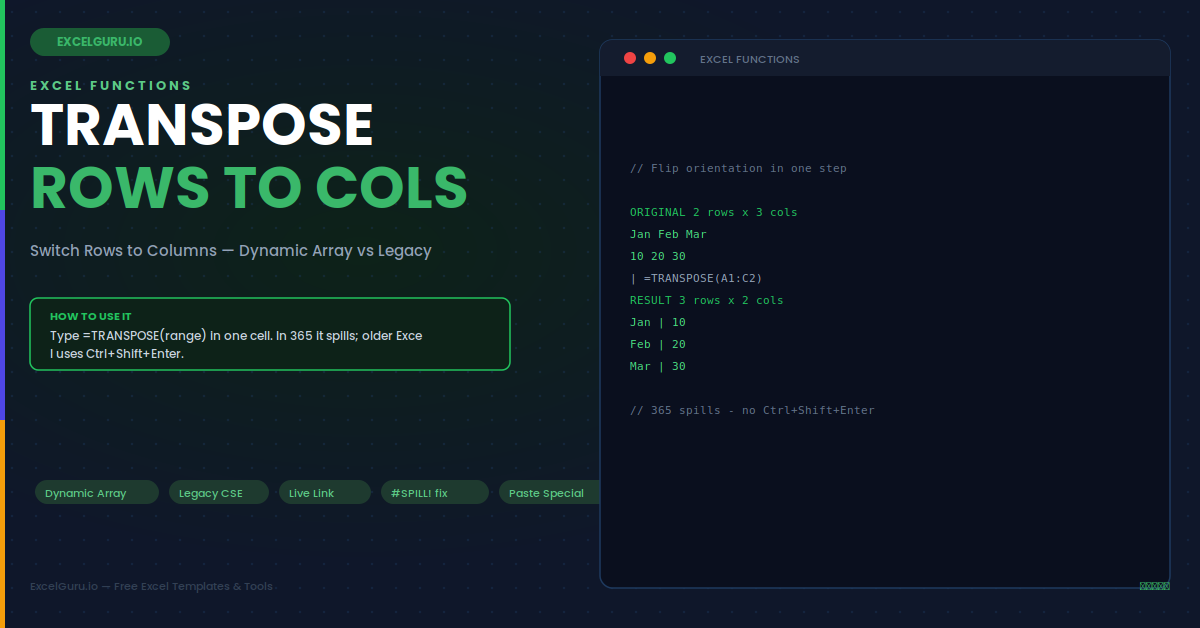
TRANSPOSE swaps the two dimensions of a cell range. In short, the rows become columns and the columns become rows. A range that is 2 rows by 3 columns becomes 3 rows by 2 columns. The top-left cell stays in place, but everything else pivots around it. The infographic below shows the flip clearly.
Notice that the values themselves do not change. Only their positions do. Specifically, the first row of the original becomes the first column of the result. This behaviour never changes, no matter how large the range is.
Dynamic Array vs Legacy — Which Method You Need
How you enter TRANSPOSE depends on your Excel version. The two methods produce the same result. However, the experience is very different. The table below compares them side by side.
| Aspect | Dynamic Array (365 / 2021) | Legacy CSE (2019 and earlier) |
|---|---|---|
| How you enter it | Type it in one cell, press Enter | Select the whole result area first, then Ctrl+Shift+Enter |
| Selecting output size | Not needed — it spills to fit | Required — you must pre-select the exact size |
| Resizing later | Automatic when the source grows | Manual — you must redo the selection |
| Formula appearance | =TRANSPOSE(A1:C2) | {=TRANSPOSE(A1:C2)} with curly braces |
The Syntax
TRANSPOSE takes just one argument. As a result, it is one of the simplest functions to remember.
Example 1: Flip a Header Row into a Column
This is the most common use. You have month names running across a row. Now you need them running down a column instead. TRANSPOSE handles it instantly.
Example 2: A Live, Linked Transpose in Excel 365
The dynamic array method keeps the result linked to the source. Therefore, edits flow through automatically. This is the key advantage over a static paste. You build it once and never touch it again.
=TRANSPOSE(A1:C4) and press Enter.Example 3: The Legacy Ctrl+Shift+Enter Method
Older Excel versions need the array-entry method. It works well, but it asks for one extra step. First you must select the output area at the correct flipped size. Then you confirm with three keys instead of one.
Example 4: Rotate a Whole Data Table
TRANSPOSE is not limited to single rows or columns. It flips entire tables just as easily. For instance, a product table with items down the side can become a table with items across the top. This is useful when a different layout suits a chart or a report.
A formula like =TRANSPOSE(A1:C3) flips this. Consequently, "Product", "Units", and "Price" move to the left column. Each item then reads across in its own column.
Example 5: Combine TRANSPOSE with Other Functions
TRANSPOSE becomes powerful when nested inside other formulas. Often you need to reorient data before a calculation. For example, you might flip a vertical list so it lines up with a horizontal one. This lets functions like SUMPRODUCT pair the values correctly.
Example 6: Static Paste vs Live Formula
Excel offers a second way to flip data: Paste Special with the Transpose option. It is quick, but it produces a frozen copy. Therefore, choosing between the two depends on whether you want the result to update. The comparison below makes the choice clear.
Example 7: Clean Up Data Pasted From a Website
Data copied from a web page often arrives in the wrong orientation. A table might paste with categories across the top when you need them down the side. TRANSPOSE fixes this without retyping. Furthermore, it pairs well with other cleanup steps. You can flip the layout first, then sort or filter the result as usual.
Troubleshooting TRANSPOSE
All three problems below are the most common. Each has a clear cause and a fast fix.
You get a #SPILL! error
This error appears in Excel 365 when something blocks the spill range. The transposed result needs empty cells to expand into. However, a value, a label, or even a stray space in the target area stops it. First, look at the cells where the result should appear. Then clear anything sitting in that block. Once the spill range is empty, the result fills in at once. Merged cells in the target area also cause this, so unmerge them if present.
The legacy result is cut off or shows #N/A
This happens when the pre-selected output area is the wrong size. The legacy method needs an exact match to the flipped dimensions. If you selected too few cells, part of the result is missing. If you selected too many, the extra cells display #N/A. To fix it, delete the formula and start again. Count the flipped size carefully: a 2x5 source needs a 5x2 selection. Then re-enter with Ctrl+Shift+Enter.
The result does not update when I change the source
If your flipped data stays frozen, you almost certainly used Paste Special instead of the formula. A transposed paste is a static copy with no link to the source. As a result, it never reflects later edits. To get live updates, replace the pasted block with a real TRANSPOSE formula. The formula keeps the connection, so every source change flows straight through to the rotated view.
Frequently Asked Questions
- How do I switch rows to columns in Excel?+Use the TRANSPOSE function. In Excel 365 or 2021, click an empty cell, type =TRANSPOSE(range) with your data range inside, and press Enter. The flipped result spills automatically into the cells below and to the right. In older versions, first select an empty area matching the flipped dimensions, type the same formula, then press Ctrl+Shift+Enter. Both methods keep the result linked to the source, so it updates whenever your original data changes. For a one-time flip with no link, use Copy then Paste Special with the Transpose option ticked instead.
- Why does TRANSPOSE give a #SPILL! error?+A #SPILL! error means the result cannot expand into the space it needs. The transposed block requires empty cells to fill. If any cell in that target area already holds a value, a label, or a stray space, Excel blocks the spill and shows the error. Clear everything in the block where the result should appear, and it will fill in immediately. Merged cells in the target area cause the same problem, so unmerge them if you find any. This error only occurs in dynamic array versions of Excel, not in the legacy method.
- What is the difference between TRANSPOSE and Paste Special Transpose?+The TRANSPOSE function creates a live result that stays linked to your source data, so it updates automatically whenever the original changes. Paste Special with Transpose creates a static, frozen copy that never updates. Choose the function when your data is still changing and the rotated view must stay in sync. Choose Paste Special when you want a quick, permanent layout change and do not need any ongoing link. The function is a formula you keep; the paste is a one-time action that produces plain values.
- Can TRANSPOSE flip an entire table, not just one row?+Yes. TRANSPOSE works on any rectangular range, whatever its size. A single row, a single column, or a full multi-column table all flip the same way. For example, =TRANSPOSE(A1:E20) rotates a 20-row, 5-column table into a 5-row, 20-column layout. The top-left cell stays in place while everything else pivots around it. In dynamic array Excel, the whole block spills automatically. In older versions, remember to select the correct flipped output size before entering the formula with Ctrl+Shift+Enter.