If you have ever used the MATCH function inside an INDEX formula, you already understand the concept behind XMATCH — it finds the position of a value in a list. But XMATCH does it better in almost every way. It defaults to exact match (so you never accidentally get the wrong result), can search from the last item rather than the first, supports wildcard partial matching with a dedicated mode, and works on both vertical and horizontal ranges without any adjustment. This guide covers the full syntax, a direct MATCH vs XMATCH comparison, and six practical examples.
XMATCH Syntax
XMATCH returns the relative position of a value in an array — a number telling you which row (or column) the match was found in.
| Argument | Required? | What it means |
|---|---|---|
| lookup_value | Required | The value to search for — a cell reference, text in quotes, or a number. |
| lookup_array | Required | The single column or single row to search in. Unlike VLOOKUP, the lookup does not need to be in a specific position — any column or row works. |
| match_mode | Optional | 0 = exact match (default — safe). -1 = exact match or next smaller. 1 = exact match or next larger. 2 = wildcard match (* and ?). |
| search_mode | Optional | 1 = search first to last (default). -1 = search last to first (finds the last match). 2 = binary search ascending. -2 = binary search descending. |
=INDEX(return_range, XMATCH(value, lookup_range)).
XMATCH vs MATCH — Key Differences
| Feature | MATCH (old) | XMATCH (new) |
|---|---|---|
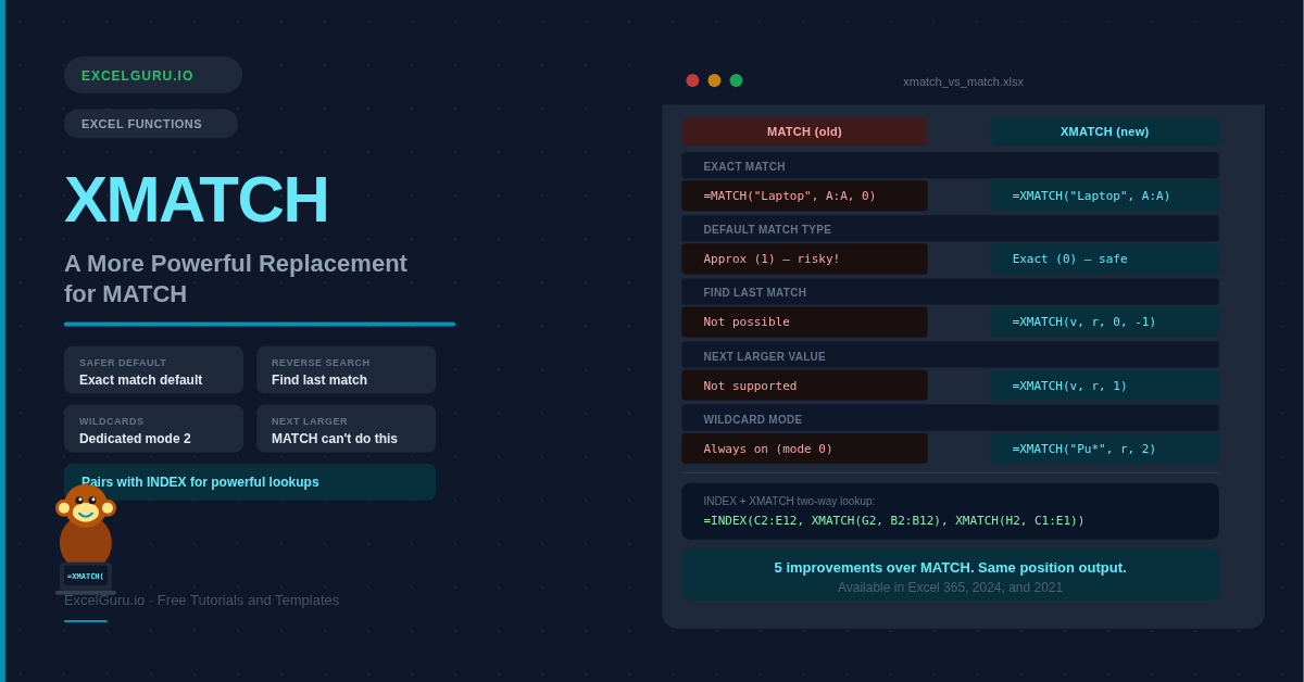
| Default match type | Approximate match (1) — dangerous on unsorted data | Exact match (0) — safe by default, no extra argument needed |
| Exact match syntax | Requires 0 as third argument: =MATCH(val, range, 0) |
Just two arguments: =XMATCH(val, range) |
| Next larger value | Not supported — only next smaller | match_mode = 1 — returns exact or next larger |
| Reverse search (last match) | Not supported — always finds first match | search_mode = -1 — finds the last match |
| Wildcard matching | Works in mode 0 — wildcards always active | Explicit mode 2 — wildcards only when you ask for them |
| Binary search | Not available | search_mode 2 or -2 — faster on large sorted datasets |
| Availability | All Excel versions | Excel 365, 2024, 2021 only |
Example 1: Basic Exact Match — Find Position in a List
In its simplest form, XMATCH needs only two arguments and returns the row number of the matching value within the lookup range. This is cleaner than MATCH because you do not need to remember to add the 0.
Example 2: INDEX + XMATCH — The Modern Lookup Combination
XMATCH by itself only returns a position number. Its real power comes when paired with INDEX — XMATCH finds the row, INDEX retrieves the value. Together they replace VLOOKUP with a formula that can look in any direction and does not break when columns are inserted.
Example 3: Reverse Search — Find the Last Occurrence
MATCH always returns the position of the first match in a list. If a value appears multiple times and you need the last one — for example, the most recent date for a repeating item — set search_mode to -1. XMATCH then searches from the bottom upward.
Example 4: Wildcard Partial Match
When you set match_mode to 2, XMATCH activates wildcard matching — * matches any sequence of characters and ? matches a single character. This is useful when you only know part of a value, such as searching for "Puma" when the list contains "Puma Co." or "Puma Ltd."
Example 5: Approximate Match — Find the Closest Value
XMATCH's match_mode -1 and 1 support approximate matching for banded ranges — useful for commission tiers, tax brackets, and discount thresholds. Unlike MATCH, XMATCH does not require sorted data for approximate matching, and it adds "next larger" support that MATCH cannot provide.
Example 6: Count Items Meeting a Threshold
Because XMATCH returns a position, you can use its approximate match modes creatively to count how many items in a sorted list fall above or below a threshold — without COUNTIF, without sorting manually, and without helper columns.
Troubleshooting XMATCH Errors
#N/A error — value not found
No item in lookup_array matches the lookup_value. Check for trailing spaces, data type mismatches (text vs number), or the value genuinely not existing. Wrap with IFERROR for a user-friendly fallback: =IFERROR(INDEX(B:B, XMATCH(E2, A:A)), "Not found").
#VALUE! error
An invalid value was passed to match_mode or search_mode. Valid match_mode values are 0, -1, 1, 2. Valid search_mode values are 1, -1, 2, -2. Any other number returns #VALUE!.
Wrong result from approximate match
Approximate match modes (-1 and 1) work most reliably on sorted data. On unsorted data, results may be unpredictable — particularly when using binary search (modes 2 and -2), which requires the array to be sorted in the matching direction. Sort your lookup array before using approximate match for guaranteed accuracy.
XMATCH not available in older Excel
You are on Excel 2019 or earlier. Use =MATCH(value, range, 0) for exact match, and consider upgrading to Microsoft 365 for the full dynamic array function suite.
Frequently Asked Questions
-
What does the XMATCH function do in Excel?+XMATCH searches for a value in a range or array and returns its relative position — a number indicating which row or column it was found in. It is the modern replacement for MATCH, with safer defaults (exact match by default), reverse search, wildcard matching, and binary search for large datasets. XMATCH is almost always paired with INDEX to retrieve an actual value from that position.
-
What is the difference between XMATCH and MATCH?+The five key improvements are: XMATCH defaults to exact match (MATCH defaults to approximate — dangerous); XMATCH can find the next larger value (MATCH cannot); XMATCH can search from last to first (MATCH cannot); XMATCH has an explicit wildcard mode so wildcards are only active when you want them; and XMATCH supports binary search for better performance on large sorted datasets. The syntax is also cleaner — exact match needs only two arguments instead of three.
-
What is the difference between XMATCH and XLOOKUP?+XLOOKUP returns a value directly — you give it a lookup value and it returns the matching item from a return range. XMATCH returns a position number — where the match was found. Use XLOOKUP for straightforward lookups where you want the result directly. Use XMATCH with INDEX when you need the position itself for further calculations, or when you want a two-way lookup that combines row and column positions.
-
Which Excel versions support XMATCH?+XMATCH is available in Microsoft 365 (all plans), Excel 2024, and Excel 2021. It is not available in Excel 2019, 2016, or any earlier version. For workbooks that need to open in older Excel, use the MATCH function instead — the results are identical for exact match scenarios, though MATCH requires an explicit 0 as the third argument.
-
How do I use XMATCH to find the last occurrence of a value?+Set search_mode to -1: =XMATCH(value, range, 0, -1). The 0 keeps exact match mode, and -1 instructs XMATCH to search from the last item upward. The result is the position of the last occurrence. Combine with INDEX to retrieve the corresponding value: =INDEX(return_range, XMATCH(value, lookup_range, 0, -1)).
-
Should I replace all my MATCH formulas with XMATCH?+For new formulas in Excel 365 or 2021, yes — XMATCH is cleaner, safer, and more capable. Do not automatically convert working MATCH formulas in existing spreadsheets unless you have a specific reason to, and never convert formulas in files shared with colleagues on Excel 2019 or older, since XMATCH will return a #NAME? error in those versions.